Policy Gradient

In RL control problems, most methods take value functions as the core learning object, improving the policy indirectly by estimating long-term returns. However, when the state or action space becomes continuous, or when the policy itself must remain stochastic, this approach becomes less direct. Policy gradient methods adopt a different perspective by treating the policy itself as the object of optimization, directly performing gradient ascent on the expected return.

The complete code for this chapter can be found in .

Policy Gradient
Parameterized Policy
The Objective
1. Episodic Tasks
2. Continuing Tasks and Average Reward
Policy Gradient Theorem
Estimating the Policy Gradient
REINFORCE：Monte Carlo Policy Gradient
Actor-Critic
Example
1. Implementation of Actor-Critic
2. Lunar Lander
Conclusion
References

Whether in Dynamic Programming (DP), Monte Carlo (MC), or Temporal Difference (TD) methods, the object learned in control problems has always been a state-value function $v_\pi(s)$ or an action-value function $q_\pi(s, a)$ . The policy is then derived and improved indirectly through these value functions.

Policy gradient methods adopt a different perspective. When the policy itself is represented as a differentiable probability distribution $\pi_\theta(a \mid s)$ , the control problem can be formulated directly as an optimization problem over the policy parameters. In this setting, rather than first estimating a value function and then improving the policy through greedy or approximately greedy procedures, one can directly perform gradient ascent on the expected return of the policy.

Through parameterized policies, the agent is able to treat the policy itself as the primary learning object, without relying on a value function as an intermediate step for policy improvement. This approach establishes a more direct connection between the learning objective and the resulting behavior, and it provides a natural modeling framework for continuous action spaces and stochastic policies.

Policy gradient methods do not negate the value of value-based approaches; instead, they offer an alternative learning pathway. Value-based methods determine behavior indirectly by estimating long-term returns, whereas Policy gradient methods attempt to directly adjust the action distribution itself, increasing the probability of actions that yield higher returns. This distinction will become evident in later sections through differences in objective function definitions, sources of gradient estimation, and the trade-offs between learning stability and variance.

Parameterized Policy

We use $\theta \in \mathbb{R}^d$ to denote the parameter vector of the policy. When the agent is at state $s$ at time step $t$ , and the current policy parameters are $\theta$ , $\pi(a \mid s, \theta)$ represents the probability of taking action $a$ in that state. Formally, this can be written as:

$\pi(a \mid s, \theta) = \text{Pr} \{ A_t = a \mid S_t = s, \theta_t = \theta \}$

After introducing a parameterized policy $\theta \in \mathbb{R}^d$ , the control problem can be transformed into a purely parameter optimization problem. Rather than directly searching for an optimal policy, we define a scalar performance objective $J(\theta)$ that takes the policy parameters as its variables, and optimize this objective by adjusting $\theta$ .

From this perspective, learning the policy can be viewed as performing gradient ascent on $J(\theta)$ . The parameter update rule can be written as:

$\theta_{t+1} = \theta_t + \widehat{\alpha \nabla J(\theta_t)}$

Here, $\widehat{\nabla J(\theta_t)}$ denotes an estimate of the true gradient, and $\alpha$ is the step size that controls the magnitude of each parameter update.

The Objective

In Policy gradient methods, control problems are reformulated as optimization problems over the policy parameters. Therefore, before deriving any parameter update rules, we must first clarify a fundamental question that is what quantity are we actually trying to maximize?

In reinforcement learning, regardless of whether a value-based or policy-based approach is adopted, the ultimate objective is always the same, that is to maximize the long-term return obtained by the agent through interaction with the environment. The differences among methods lie not in the learning objective itself, but in how the return is formalized and optimized.

Because Policy gradient methods directly adjust the policy parameters, the learning objective must be expressed as a scalar function that is differentiable with respect to $\theta$ . This function is typically denoted as $J(\theta)$ and is used to measure the overall performance of the agent under the policy $\pi_\theta$ . Depending on whether the task is episodic or continuing, and on whether a discount factor is introduced, the specific definition of $J(\theta)$ may vary. Nevertheless, its underlying meaning remains the same: the expected amount of return accumulated under the current policy.

Once $J(\theta)$ is clearly defined, we can proceed to discuss its gradient form and derive practical policy update rules.

Episodic Tasks

In episodic tasks, each interaction between the agent and the environment terminates after a finite number of time steps. Under this setting, the return can be defined as the discounted return accumulated from time step $t$ until the end of the episode:

$\displaystyle G_t \doteq \sum_{k=0}^{T-t-1} \gamma^k R_{t+k+1}$

where $T$ denotes the termination time of the episode.

For a parameterized policy $\pi_\theta$ , the objective of Policy Gradient methods can be defined as the state-value of the initial state:

$J(\theta) \doteq v_{\pi_\theta}(s_0) = \mathbb{E}_{\pi_\theta}[G_0]$

That is, under the policy $\pi_\theta$ , the objective measures the expected accumulated return obtained by the agent starting from the initial state $s_0$ .

Conceptually, this definition is equivalent to maximizing the initial-state value $v_\pi(s_0)$ in value-based methods. The difference lies only in the optimization variable: Policy gradient methods optimize the policy parameters $\theta$ , rather than the value function itself.

Continuing Tasks and Average Reward

In continuing tasks, the interaction between the agent and the environment does not terminate naturally, and therefore there is no explicit episode boundary. Under this setting, in addition to using discounted return as a performance measure, another commonly used and more long-term–oriented criterion is the average reward.

For a given policy $\pi$ , the average reward can be defined as the expected return obtained per time step over an infinite time horizon:

$\displaystyle r(\pi) \doteq \lim_{T \to \infty} \frac{1}{T} \mathbb{E} \Big[ \sum_{t=1}^{T} R_t \mid S_0, A_{0:t-1} \sim \pi \Big]$

This definition characterizes the steady-state performance of the agent over long-term operation, rather than the accumulated return of a single episode.

If we further assume that, under policy $\pi$ , the system admits a stationary distribution $\mu_\pi(s)$ , the average reward can equivalently be expressed as an expectation over states and actions:

$\displaystyle r(\pi) = \sum_s \mu_\pi(s) \sum_a \pi(a \mid s, \theta) \sum_{s^\prime, r} p(s^\prime, r \mid s, a) r$

In continuing tasks, the objective function of Policy gradient methods is defined as this long-term average reward, namely,

$J(\theta) \doteq r(\pi_\theta)$

The goal of policy learning is therefore to adjust the parameters $\theta$ so as to maximize the average reward under the steady-state behavior induced by the policy.

Compared with discounted return, the average reward does not depend on a discount factor $\gamma$ , and thus more directly reflects the stable long-term performance of a policy. This makes it particularly suitable for tasks that run continuously and do not have natural termination conditions. However, the analysis of average reward typically relies on the existence of a stationary distribution, which also makes its theoretical treatment and practical implementation more involved. In later policy gradient derivations, these two objective formulations will lead to different gradient expressions, but they share the same core idea, that is adjusting the policy so that high-return behaviors occur more frequently in the long run.

Policy Gradient Theorem

Policy gradient methods exhibit a highly consistent mathematical structure under both episodic and continuing task settings. The difference lies only in the presence of a time-scale–dependent proportional constant, which does not affect the direction of the gradient.

For episodic tasks, the policy gradient can be written in the following form:

$\displaystyle \nabla J(\theta) \propto \sum_s \mu(s) \sum_a \nabla \pi(a \mid s) q_\pi(s, a)$

Here, $\mu(s)$ denotes the expected number of times that state $s$ is visited within an episode under the current policy $\pi$ . In other words, $\mu(s)$ reflects the relative importance of that state to the overall return. The proportionality symbol $\propto$ indicates that, in the episodic setting, the direction of the policy gradient is determined by this expression, while the constant scaling factor does not affect the direction of gradient ascent.

For continuing tasks, the policy gradient Theorem can be written as an exact equality:

$\displaystyle \nabla J(\theta) = \sum_s \mu(s) \sum_a \nabla \pi(a \mid s) q_\pi(s, a)$

In this case, $\mu(s)$ represents the state visitation weighting under policy $\pi$ . In the discounted setting, it corresponds to the discounted state visitation measure; in the average-reward setting, it corresponds to the stationary distribution of the system. As in the episodic case, the mechanism of policy update remains the same, that is within each state, action selection probabilities are adjusted according to the importance of that state.

From an operational perspective, the above expression shows that the policy gradient is formed by aggregating contributions from all states, where the weight of each state is given by its visitation frequency $\mu(s)$ under the current policy. In a particular state $s$ , changes in the policy probability for an action $a$ , given by $\nabla \pi(a \mid s)$ , are weighted by the action value $q_\pi(s, a)$ . Actions with higher value therefore contribute more strongly to the gradient.

Regardless of whether the task is episodic or continuing, the policy gradient theorem reveals several key facts:

Policy improvement is performed on a per-state basis.
- The overall change of the policy can be decomposed into local adjustments of action probabilities within each state.
The improvement direction depends only on the action-value function .
- High-value actions have their probabilities increased, while low-value actions have their probabilities decreased.
State importance is naturally weighted by .
- States that are visited more frequently, or that have a greater impact on long-term performance, contribute more to the overall gradient.
No differentiation through the environment dynamics is required.
- The computation of the policy gradient does not involve gradients of state transition probabilities or an explicit environment model.

The policy gradient theorem thus provides an analytic expression for $\nabla J(\theta)$ . Substituting this result back into the update rule for a parameterized policy yields the learning rule for the policy parameters:

$\theta_{t+1} = \theta_t + \alpha \nabla J(\theta_t)$

The significance of the policy gradient theorem lies in its transformation of the gradient of the overall expected return into a form that depends only on the policy itself and the action values. Although the expression still involves unknown quantities such as $q_\pi(s, a)$ and $\mu(s)$ , its structure makes it clear that, as long as these quantities can be approximated from sampled data, policy learning can proceed without explicitly modeling the environment dynamics. The following sections will further show how, through the log-derivative trick, this expression can be converted into an update rule that can be estimated directly from sampled trajectories.

Estimating the Policy Gradient

Although the policy gradient theorem provides an analytic expression for the policy gradient, this formula cannot be computed directly in practice, because it contains several quantities that are unknown or unavailable:

$\mu(s)$ : the visitation probability (or visitation weight) of each state under the current policy is generally unknown.
$q_\pi(s, a)$ : the true expected return of each state–action pair cannot be obtained in advance.
The expression itself requires summation over all state–action pairs, which is infeasible in large-scale or continuous state spaces.

To address these difficulties, policy gradient methods exploit trajectory samples generated through actual interaction with the environment to simultaneously approximate $\mu(s)$ and $q_\pi(s, a)$ , thereby constructing an unbiased (or low-bias) estimator of $\nabla J(\theta)$ .

We begin with the policy gradient Theorem and reorganize the gradient term. For any state $s$ and action $a$ , we have:

$\begin{aligned} \nabla J(\theta) &= \sum_s \mu(s) \sum_a \nabla \pi(a \mid s, \theta) q_\pi(s, a) \\ &= \sum_s \mu(s) \sum_a \pi(a \mid s, \theta) \frac{1}{\pi(a \mid s, \theta)} \nabla \pi(a \mid s, \theta) q_\pi(s, a) \\ &= \sum_s \mu(s) \sum_a \frac{\nabla \pi(a \mid s, \theta)}{\pi(a \mid s, \theta)} q_\pi(s, a) \\ &= \sum_s \mu(s) \sum_a \nabla \ln \pi(a \mid s, \theta) q_\pi(s, a) \end{aligned}$

This step makes use of the log-derivative identity:

$\displaystyle \nabla \ln \pi(a \mid s, \theta) = \frac{\nabla \pi(a \mid s, \theta)}{\pi(a \mid s, \theta)}$

The significance of this transformation is that the gradient of the policy can be expressed as the gradient of the log-probability of the policy, a quantity that depends only on the policy itself.

Interpreting the double summation as an expectation under the distribution $S \sim \mu, A \sim \pi$ , we obtain:

$\nabla J(\theta) = \mathbb{E}_{S \sim \mu, A \sim \pi} \Big[ \nabla \ln \pi(A \mid S) q_\pi(S, A) \Big]$

This expression reveals that we do not need to explicitly compute $\mu(s)$ or enumerate all states. As long as the agent interacts with the environment according to the current policy, states will naturally appear according to the distribution $\mu$ , and actions will be selected according to $\pi$ . In other words, the sampling process itself implicitly carries out the computation of $\sum_s \mu(s) \sum_a \pi(a \mid s)$ .

Based on this expectation form, the update of the policy parameters $\theta$ can be rewritten in a sampled approximation as:

$\theta_{t+1} \leftarrow \theta_t + \alpha \widehat{\nabla J(\theta_t)} = \theta_t + \alpha \nabla \ln \pi(A_t \mid S_t,\theta) \hat{q}(S_t,A_t)$

Here, $\hat{q}(S_t, A_t)$ denotes an estimate of the true action-value $q_\pi(S_t, A_t)$ , which in practice can be obtained from MC returns, TD estimates, or other approximation methods.

The above derivation shows that the estimation error of the policy gradient mainly arises from two sources: the stochastic variance induced by finite sampling, and the approximation error in estimating $q_\pi(s, a)$ . Subsequent methods, such as REINFORCE and Actor–Critic, address these issues by adopting different strategies to estimate or approximate this return term, thereby trading off bias and variance.

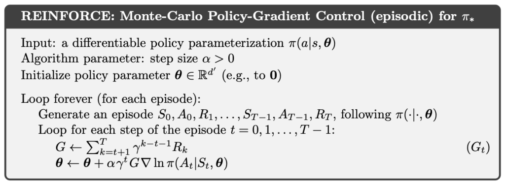
REINFORCE：Monte Carlo Policy Gradient

REINFORCE refers to a policy gradient method that directly estimates the action-value function $q_\pi(s, a)$ using MC returns. The central idea is to use the return actually observed along a complete trajectory as an approximation of the return term in the policy gradient.

Consider a state–action pair $(S_t, A_t)$ occurring at time step $t$ . By following the policy $\pi$ until the episode terminates, the MC method defines the return by accumulating all subsequent rewards:

$\displaystyle G_t = \sum_{k=0}^{T-t-1} \gamma^k R_{t+k+1}$

In the episodic setting, for a given $(s, a)$ , the action-value function can be written as:

$q_\pi(s, a) = \mathbb{E}_\pi [ G_t \mid S_t=s, A_t=a ]$

Therefore, the return $G_t$ obtained from actual interaction can be regarded as an unbiased sample of $q_\pi(s, a)$ .

At the implementation level, the MC method accomplishes two tasks simultaneously through the generated trajectory. First, the observed pairs $(S_t, A_t)$ approximate the state–action distribution induced by the policy $\pi$ . Second, the observed return $G_t$ serves as an estimate of $q_\pi(s, a)$ . As a result, the expectation in the policy gradient formulation can be approximated directly by a sample average.

Combining this with the previous derivation of policy gradient estimation, the policy gradient ascent update rule for REINFORCE can be written as:

$\theta_{t+1} \leftarrow \theta_t + \alpha G_t \nabla_\theta \ln \pi_\theta(A_t \mid S_t)$

REINFORCE thus constitutes a policy gradient method that uses MC returns as an unbiased estimator of $q_\pi(s, a)$ . Because it completely avoids bootstrapping, its theoretical structure is clean and conceptually straightforward. However, precisely because it relies on the return from an entire trajectory as the learning signal, the resulting policy gradient estimates typically exhibit very high variance, which in practice can lead to unstable learning or slow convergence.

The complete REINFORCE algorithm is as below:

REINFORCE: Monte-Carlo Policy-Gradient Control (episodic) (source: Reinforcement Learning: An Introduction, 2nd).

Actor-Critic

The main limitation of REINFORCE lies in the high variance of its gradient estimates, as well as the fact that updates can only be performed after an entire episode has terminated, which prevents true online learning. Actor–Critic methods address this issue by introducing a Critic trained with a TD method that can be learned online. The Critic estimates the state value and provides a TD signal at every time step, which is then used to update the policy (Actor) without waiting for episode termination.

With this design, Actor–Critic trades bootstrapping for lower variance and the ability to perform online updates, at the cost of introducing bias relative to REINFORCE. This trade-off between bias and variance is the central design choice of Actor–Critic methods.

An Actor–Critic method consists of two components that are learned simultaneously:

The Actor represents and updates the policy $\pi(a \mid s, \theta)$ , with the objective of maximizing the policy performance measure $J(\theta)$ .
The Critic is responsible for learning the state-value function $v_\pi(s, \mathbf{w})$ under the current policy $\pi$ , and for providing an immediate evaluation signal of the quality of the current behavior, which is used to guide the Actor’s policy updates.

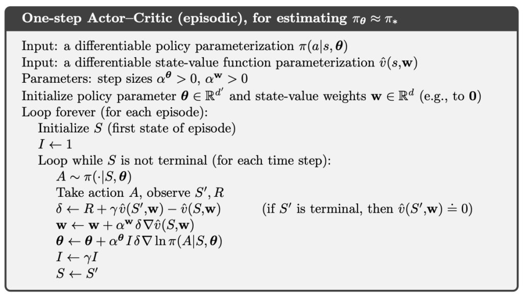
The Critic is typically trained using TD learning. In the simplest one-step setting, the Critic uses TD(0) to update its value function estimate:

$\delta_t = R_{t+1} + \gamma v_\mathbf{w}(S_{t+1}) - v_{\mathbf{w}}(S_t) \\\\ \mathbf{w} \leftarrow \mathbf{w} + \beta \delta_t \nabla_{\mathbf{w}} v_{\mathbf{w}}(S_t)$

where $\delta_t$ denotes the TD error, which reflects the discrepancy between the current value estimate and the one-step bootstrapped target.

The Actor uses the TD error provided by the Critic as an approximation of the return term in the policy gradient, and updates the policy parameters immediately:

$\theta \leftarrow \theta + \alpha \delta_t \nabla_\theta \ln \pi_\theta(A_t \mid S_t)$

From the policy gradient perspective, the TD error plays the role of an instantaneous return signal. When the observed return is better than expected (i.e., $\delta_t > 0$ ), the Actor increases the probability of selecting the current action; conversely, when the outcome is worse than expected, the probability is decreased.

Within the unified framework of the policy gradient Theorem, the difference between Actor–Critic and REINFORCE can be clearly understood in terms of how $q_\pi(s, a)$ is estimated:

REINFORCE uses the full MC return as an unbiased estimator of $q_\pi(s, a)$ , but suffers from high variance and cannot perform online updates.
Actor–Critic uses a value function trained via TD learning, and employs the TD error for bootstrapping, introducing bias in exchange for lower variance and the ability to update online.

As a result, Actor–Critic methods allow policy gradient approaches to be applied effectively to long-horizon or continuing tasks, rather than being restricted to episodic settings.

The complete One-Step Actor–Critic algorithm is as below:

One-step Actor–Critic (episodic) (source: Reinforcement Learning: An Introduction, 2nd).

Example

Implementation of Actor-Critic

In this implementation, both the Actor and the Critic use multi-layer perceptrons (MLPs) as function approximators. The Actor network outputs logits for each action and samples from a Categorical distribution to form a stochastic policy $\pi_\theta(a \mid s)$ . The Critic, on the other hand, estimates the state value $v(s)$ , which serves as the baseline for TD learning.

At each time step of interaction, the training procedure proceeds as follows. First, the Critic computes the TD target based on the current and next states, and then obtains the TD error. The Critic updates its value function parameters by minimizing the squared TD error, allowing $v(s)$ to gradually approximate the true state-value under the current policy.

The Actor uses the same TD error as the learning signal for policy updates. This signal is multiplied by the log-probability of the selected action, $\log \pi_\theta(a \mid s)$ , to form an estimate of the policy gradient. In implementation, the TD error is detached when used for the Actor update, preventing gradients from flowing back to the Critic through the Actor’s loss. This ensures that the Critic is updated solely through its own TD learning process. Conceptually, this treatment corresponds to the semi-gradient setting in the policy gradient theorem.

To improve overall training stability, different learning rates are used for the Actor and the Critic to reflect their distinct learning dynamics. In addition, gradient clipping is applied to both networks to prevent training instability caused by exploding gradients.

import numpy as np
import torch
import torch.nn as nn
from torch import optim


class Actor(nn.Module):
    def __init__(self, observation_dim: int, n_actions: int, hidden_dim: int = 256):
        super().__init__()
        self.network = nn.Sequential(
            nn.Linear(observation_dim, hidden_dim),
            nn.Tanh(),
            nn.Linear(hidden_dim, hidden_dim),
            nn.Tanh(),
            nn.Linear(hidden_dim, n_actions),
        )

    def forward(self, obs: torch.Tensor):
        logits = self.network(obs)
        return torch.distributions.Categorical(logits=logits)


class Critic(nn.Module):
    def __init__(self, observation_dim: int, hidden_dim: int = 256):
        super().__init__()
        self.critic = nn.Sequential(
            nn.Linear(observation_dim, hidden_dim),
            nn.Tanh(),
            nn.Linear(hidden_dim, hidden_dim),
            nn.Tanh(),
            nn.Linear(hidden_dim, 1),
        )

    def forward(self, obs: torch.Tensor):
        return self.critic(obs).squeeze(-1)


class ActorCritic(nn.Module):
    def __init__(
        self,
        observation_dim: int,
        n_actions: int,
        *,
        hidden_dim: int,
        actor_lr: float = 1e-4,
        critic_lr: float = 1e-3,
        grad_clip=2.0,
        gamma: float = 0.99,
    ):
        super().__init__()
        self.actor = Actor(observation_dim, n_actions, hidden_dim)
        self.critic = Critic(observation_dim, hidden_dim)
        self.grad_clip = grad_clip
        self.gamma = gamma
        self.actor_optimizer = optim.Adam(self.actor.parameters(), lr=actor_lr)
        self.critic_optimizer = optim.Adam(self.critic.parameters(), lr=critic_lr)

    def act(self, s: np.ndarray):
        s_t = torch.tensor(s, dtype=torch.float32).unsqueeze(0)
        pi_s = self.actor(s_t)
        a = pi_s.sample()
        return int(a.item()), pi_s

    def update(
        self, s: np.ndarray, a: int, r: float, s_prime: np.ndarray, pi_s: torch.distributions.Categorical, terminated: bool
    ) -> tuple[float, float]:
        s_t = torch.tensor(s, dtype=torch.float32).unsqueeze(0)
        a_t = torch.tensor([a], dtype=torch.long).unsqueeze(0)
        s_tp1 = torch.tensor(s_prime, dtype=torch.float32).unsqueeze(0)
        v_t = self.critic(s_t)

        with torch.no_grad():
            if terminated:
                v_prime = torch.tensor(0.0)
            else:
                v_prime = self.critic(s_tp1)
            td_target = r + self.gamma * v_prime

        td_error = td_target - v_t

        critic_loss = 0.5 * td_error.pow(2)
        self.critic_optimizer.zero_grad()
        critic_loss.backward()
        nn.utils.clip_grad_norm_(self.critic.parameters(), self.grad_clip)
        self.critic_optimizer.step()

        actor_loss = -(td_error.detach() * pi_s.log_prob(a_t))
        self.actor_optimizer.zero_grad()
        actor_loss.backward()
        nn.utils.clip_grad_norm_(self.actor.parameters(), self.grad_clip)
        self.actor_optimizer.step()

        return float(actor_loss.item()), float(critic_loss.item())

Lunar Lander

LunarLander is a classic rocket-trajectory optimization problem. According to Pontryagin’s maximum principle, under an optimal policy the engine is either fired at full thrust or kept completely off. Accordingly, this environment uses a discrete action space, where each action corresponds to turning an engine on or off.

The action space contains four actions:

0: Do nothing.
1: Fire the left engine.
2: Fire the main engine.
3: Fire the right engine.

Each state is an 8-dimensional vector consisting of:

The lander’s x and y position.
The lander’s x and y linear velocity.
The lander’s angle.
The lander’s angular velocity.
Two boolean values indicating whether the left and right legs are in contact with the ground.

At each time step, the reward is shaped as follows:

The closer the lander is to the landing pad, the higher the reward; the farther away, the lower the reward.
The slower the lander is moving, the higher the reward; the faster it is moving, the lower the reward.
The more the lander is tilted, the lower the reward.
A bonus of +10 is given for each leg that is in contact with the ground.
A penalty of −0.03 is applied for each frame in which a side engine fires.
A penalty of −0.3 is applied for each frame in which the main engine fires.

When an episode terminates by either crashing or landing safely, an additional terminal reward is given:

Crash: −100.
Safe landing: +100.

An episode is considered solved if its total reward reaches 200 or higher.

In the following code, we train Actor-Critic for 1000 episodes.

import time

import gymnasium as gym

from actor_critic import ActorCritic

GYM_ID = "LunarLander-v3"
N_EPISODES = 1000
MAX_STEPS = 1000


def play_game(agent: ActorCritic, episodes=1):
    visual_env = gym.make(GYM_ID, render_mode="human")  # UI window

    for episode in range(episodes):
        state, _ = visual_env.reset()
        terminated = False
        truncated = False
        total_reward = 0.0
        step_count = 0

        input("Press Enter to play game")

        print(f"Episode {episode + 1} starts")
        while not terminated and not truncated:
            action, _ = agent.act(state)
            state, reward, terminated, truncated, _ = visual_env.step(action)
            total_reward += reward
            step_count += 1
            visual_env.render()

        print(f"Episode {episode + 1} is finished: Total reward is {total_reward}, steps = {step_count}")
        time.sleep(1)

    visual_env.close()


def train() -> ActorCritic:
    env = gym.make(GYM_ID)
    agent = ActorCritic(
        observation_dim=env.observation_space.shape[0],
        n_actions=env.action_space.n,
        hidden_dim=256,
        actor_lr=3e-4,
    )

    returns = 0.0

    for i_episode in range(1, N_EPISODES + 1):
        print(f"\rEpisode: {i_episode}/{N_EPISODES}", end="", flush=True)

        s, _ = env.reset()
        done = False
        G = 0.0
        steps = 0

        while not done and steps < MAX_STEPS:
            a, pi_s = agent.act(s)
            s_prime, r, terminated, truncated, _ = env.step(a)
            G += r
            done = terminated or truncated
            agent.update(s, a, r, s_prime, pi_s, done)
            s = s_prime
            steps += 1

        returns += G
        if i_episode % 50 == 0:
            print(f"\nEpisode: {i_episode}/{N_EPISODES}, average return: {returns / 50:.2f}")
            returns = 0.0

    return agent


if __name__ == "__main__":
    agent = train()
    play_game(agent)

After training for approximately 1,000 episodes, the Actor–Critic agent is able to complete the landing task reliably. During execution, the lander is observed to remain mostly above the landing pad, with lateral displacement well controlled, and to descend gradually at a smooth and continuous rate until a successful touchdown is achieved.

This behavior indicates that, by using the TD error as an immediate learning signal, the Actor–Critic method is able to learn smooth and stable control policies. Compared with learning approaches that rely on full-episode returns and tend to produce large, abrupt corrections, the policy updates in Actor–Critic are more incremental, favoring adjustments that maintain stable posture and position. This also reflects the natural preference of on-policy Actor–Critic methods for learning stability and safe behavior in continuous control problems.

Lunar Lander by Actor-Critic with 1000 episodes.

Conclusion

By contrasting REINFORCE and Actor–Critic, we can clearly see the trade-offs that policy gradient methods make between bias and variance, as well as the impact of bootstrapping and online update capability on control stability. The experimental results show that, by using the TD error as an immediate learning signal, Actor–Critic is able to learn continuous and smooth control behaviors, enabling policy gradient methods to be applied effectively to long-horizon and continuous control tasks. Overall, policy gradient methods not only offer an alternative learning pathway to value-based approaches, but also establish a clear and consistent theoretical foundation for more advanced control and deep reinforcement learning methods that follow.

References

Adam White and Martha White. Reinforcement Learning Specialization. University of Alberta and Coursera.
Richard S. Sutton and Andrew G. Barto. 2020. Reinforcement Learning: An Introduction, 2^nd. The MIT Press.

Policy Gradient

Share

Table of Contents

Policy Gradient

Parameterized Policy

The Objective

Episodic Tasks

Continuing Tasks and Average Reward

Policy Gradient Theorem

Estimating the Policy Gradient

REINFORCE：Monte Carlo Policy Gradient

Actor-Critic

Example

Implementation of Actor-Critic

Lunar Lander

Conclusion

References

Related Tags

Leave a Reply Cancel reply

You May Also Like