
CLIP (Contrastive Language-Image Pre-training) is a model proposed by OpenAI in 2021. It achieves strong generalization capability by integrating visual and language representations, and it has extensive potential applications. This article will introduce both the theory and practical implementation of CLIP.
The complete code for this chapter can be found in .
Architecture
OpenAI introduced the CLIP model in 2021. The motivation behind its design stems from the limitations of traditional image classification models, which rely on fixed labels and thus lack generalization ability. To overcome this constraint, CLIP adopts a novel pre-training approach: contrastive learning. It learns a joint embedding space for vision and language by leveraging a large dataset of image-text pairs. This enables CLIP to demonstrate impressive zero-shot generalization to tasks it was never explicitly trained on.
CLIP jointly trains an image encoder and a text encoder to learn a multi-modal embedding space. The training objective is to maximize the cosine similarity between embeddings of matching image-text pairs, while minimizing the similarity between mismatched pairs. These similarity scores are optimized using a symmetric cross-entropy loss.
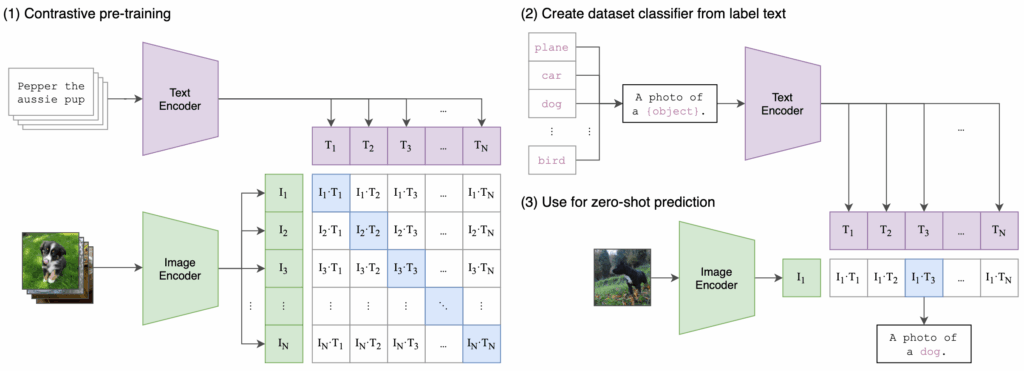
The following pseudo code illustrates how, during pre-training, the text and image embeddings are used to compute the loss.
# image_encoder - ResNet or Vision Transformer
# text_encoder - CBOW or Text Transformer
# I[n, h, w, c] - minibatch of aligned images
# T[n, l] - minibatch of aligned texts
# W_i[d_i, d_e] - learned proj of image to embed
# W_t[d_t, d_e] - learned proj of text to embed
# t - learned temperature parameter
# extract feature representations of each modality
I_f = image_encoder(I) #[n, d_i]
T_f = text_encoder(T) #[n, d_t]
# joint multimodal embedding [n, d_e]
I_e = l2_normalize(np.dot(I_f, W_i), axis=1)
T_e = l2_normalize(np.dot(T_f, W_t), axis=1)
# scaled pairwise cosine similarities [n, n]
logits = np.dot(I_e, T_e.T) * np.exp(t)
# symmetric loss function
labels = np.arange(n)
loss_i = cross_entropy_loss(logits, labels, axis=0)
loss_t = cross_entropy_loss(logits, labels, axis=1)
loss = (loss_i + loss_t)/2
Text Encoder
CLIP’s text encoder is based on the Transformer encoder architecture. If you’re not yet familiar with the Transformer, please refer to the following article first.

CLIP uses the following parameter settings:
- Layers: 12
- Attention heads: 8
- d_model: 512
- Tokenizer: Byte Pair Encoding (BPE)
- Vocab size: 49152
- Max sequence length: 76
- Total parameters: 63M
Additionally, CLIP applies some modifications to the Transformer encoder. These modifications are inspired by the adjustments made in GPT to the Transformer decoder—for example, placing the LayerNorm before each sub-block (a pre-LN architecture).
The text encoder wraps the input text sequence with [SOS] and [EOS] tokens, and uses the activation at the [EOS] position from the final layer of the Transformer encoder as the feature representation of the text.
OpenAI has open-sourced the code for CLIP, which can be found here. The following implementation of the text encoder is a simplified version rewritten based on the official source code.
import torch
import torch.nn as nn


class ResidualAttentionBlock(nn.Module):
    def __init__(self, d_model, n_head):
        super().__init__()
        self.attn = nn.MultiheadAttention(d_model, n_head)
        self.ln_1 = nn.LayerNorm(d_model)
        self.mlp = nn.Sequential(
            nn.Linear(d_model, d_model * 4),
            nn.GELU(),
            nn.Linear(d_model * 4, d_model)
        )
        self.ln_2 = nn.LayerNorm(d_model)

    def forward(self, x):
        """
        Parameters
        ----------
        x: Tensor of shape [batch_size, sequence_length, d_model]
        """
        attn_out, _ = self.attn(self.ln_1(x), self.ln_1(x), self.ln_1(x))
        x = x + attn_out
        x = x + self.mlp(self.ln_2(x))
        return x


class Transformer(nn.Module):
    def __init__(self, width, layers, heads):
        super().__init__()
        self.resblocks = nn.Sequential(
            *[ResidualAttentionBlock(width, heads) for _ in range(layers)]
        )

    def forward(self, x):
        return self.resblocks(x)


class TextEncoder(nn.Module):
    def __init__(self, vocab_size, context_length, width, layers, heads):
        super().__init__()
        self.token_embedding = nn.Embedding(vocab_size, width)
        self.positional_embedding = nn.Parameter(torch.empty(context_length, width))
        nn.init.normal_(self.positional_embedding, std=0.01)
        self.transformer = Transformer(width, layers, heads)
        self.ln_final = nn.LayerNorm(width)
        self.context_length = context_length

    def forward(self, text):
        """
        Parameters
        ----------
        text: Tensor of shape [batch_size, context_length] containing token indices.
        """

        x = self.token_embedding(text)  # [batch_size, context_length, width]
        x = x + self.positional_embedding
        x = x.permute(1, 0, 2)  # [context_length, batch, width]
        x = self.transformer(x)
        x = x.permute(1, 0, 2)  # [batch, context_length, width]
        x = self.ln_final(x)
        return x[:, -1, :]  # [batch, width]
Image Encoder
In the CLIP paper, OpenAI compared the performance of five image encoders based on ResNets and three based on Vision Transformers (ViTs). These are as follows:
- ResNet-50
- ResNet-101
- RN50x4: ResNet-50 scaled up by 4×
- RN50x16: ResNet-50 scaled up by 16×
- RN50x64: ResNet-50 scaled up by 64×
- ViT-B/32
- ViT-B/16
- ViT-L/14
In the zero-shot performance evaluation presented in the paper, the Vision Transformer (ViT) architecture outperformed the CNN-based ResNet models. Among the three ViT models, ViT-L/14 achieved the best performance, followed by ViT-B/16 and then ViT-B/32. This demonstrates the excellent generalization capability of Vision Transformers when trained on large-scale data.
In the official CLIP codebase, the authors implement the Vision Transformer directly. In the following code, we use vit_b_16 from torchvision. In the constructor, we remove the classification head of the vit_b_16 model.
from torchvision.models import vit_b_16, ViT_B_16_Weights


class ImageEncoder(nn.Module):
    def __init__(self, output_dim=512):
        super().__init__()
        self.vit = vit_b_16(weights=ViT_B_16_Weights.IMAGENET1K_V1)
        self.vit.heads = nn.Identity()  # [batch, 768]
        self.proj = nn.Linear(self.vit.hidden_dim, output_dim)

    def forward(self, x):
        features = self.vit(x)  # [batch, 768]
        features = self.proj(features)  # [batch, output_dim]
        return features
CLIP
The following code integrates the previously described text and image encoders into a complete CLIP implementation. As you can see, this code is essentially a practical implementation of the earlier pseudo code.
class CLIP(nn.Module):
    def __init__(self, image_embed_dim, text_vocab_size, context_length, text_width, text_layers, text_heads):
        super().__init__()
        self.image_encoder = ImageEncoder(image_embed_dim)
        self.text_encoder = TextEncoder(text_vocab_size, context_length, text_width, text_layers, text_heads)
        self.logit_scale = nn.Parameter(torch.ones([]) * torch.log(torch.tensor(1 / 0.07)))

    def encode_image(self, image):
        return self.image_encoder(image)

    def encode_text(self, text):
        return self.text_encoder(text)

    def forward(self, image, text):
        image_features = F.normalize(self.encode_image(image), dim=-1)
        text_features = F.normalize(self.encode_text(text), dim=-1)
        logit_scale = self.logit_scale.exp()
        logits_per_image = logit_scale * image_features @ text_features.t()
        logits_per_text = logits_per_image.t()
        return logits_per_image, logits_per_text
The code below demonstrates how to use CLIP in practice.
if __name__ == "__main__":
    vocab_size = 49408
    context_length = 77
    image_embed_dim = 512
    text_width = 512
    text_layers = 12
    text_heads = 8

    model = CLIP(
        image_embed_dim=image_embed_dim,
        text_vocab_size=vocab_size,
        context_length=context_length,
        text_width=text_width,
        text_layers=text_layers,
        text_heads=text_heads
    )

    batch_size = 2
    image = torch.randn(batch_size, 3, 224, 224)
    text = torch.randint(0, vocab_size, (batch_size, context_length))

    logits_per_image, logits_per_text = model(image, text)
    print("logits_per_image shape:", logits_per_image.shape)
    print("logits_per_text shape:", logits_per_text.shape)
Applications
Since CLIP embeds both images and text into the same vector space, it enables cross-modal retrieval. One of the most direct applications is visual search, which includes the following three tasks:
- Image-to-Image Search: Given an input image, retrieve similar images.
- Image-to-Text Search: Given an input image, retrieve relevant texts.
- Text-to-Image Search: Given an input text, retrieve similar images.
Example
We will use CLIP to implement an image-to-image search. In this example, we have 5 product images each for electric fans, refrigerators, and washing machines.
First, we use CLIP’s image encoder to convert these 15 product images into embeddings.
import os
from pathlib import Path

import clip
import faiss
import numpy as np
import torch
from PIL import Image

device = "cuda" if torch.cuda.is_available() else "cpu"
model, preprocess = clip.load("ViT-B/32", device=device)

PRODUCT_IMAGES = Path(__file__).parent.parent / "product_images"


def build_database_embeddings(database_folder):
    image_files = [f for f in os.listdir(database_folder) if f.endswith(('.jpg', '.jpeg', '.png'))]
    embeddings = []
    filenames = []

    for img_file in image_files:
        img_path = os.path.join(database_folder, img_file)
        image = preprocess(Image.open(img_path)).unsqueeze(0).to(device)

        with torch.no_grad():
            embedding = model.encode_image(image).cpu().numpy()

        embeddings.append(embedding / np.linalg.norm(embedding))
        filenames.append(img_file)

    embeddings = np.vstack(embeddings).astype('float32')
    return embeddings, filenames


print("Building database embeddings...")
db_embeddings, filenames = build_database_embeddings(PRODUCT_IMAGES)
Next, we add these embeddings to a FAISS index. Of course, you can use other vector databases such as ChromaDB or Milvus.
def build_faiss_index(embeddings):
    dimension = embeddings.shape[1]
    index = faiss.IndexFlatIP(dimension)  # Inner product similarity
    index.add(embeddings)
    return index


print("Creating FAISS index...")
faiss_index = build_faiss_index(db_embeddings)
Finally, we want to find images that are similar to a given SEARCH_IMAGE.
def search_similar_product(user_image_path, index, filenames):
    image = preprocess(Image.open(user_image_path)).unsqueeze(0).to(device)

    with torch.no_grad():
        query_embedding = model.encode_image(image).cpu().numpy()

    query_embedding /= np.linalg.norm(query_embedding)
    distances, indices = index.search(query_embedding, k=3)
    return [(filenames[i], distances[0][idx]) for idx, i in enumerate(indices[0])]


SEARCH_IMAGE = "./search-image-1.jpg"

print("Searching for similar products...")
results = search_similar_product(SEARCH_IMAGE, faiss_index, filenames)

print("Top matched products:")
for filename, score in results:
    print(f"Product: {filename}, Similarity Score: {score:.4f}")
Conclusion
CLIP is like teaching a computer to both see images and read text, enabling it not only to understand pictures but also to accurately connect them with textual descriptions. With this powerful capability, we can more easily develop a wide range of applications that involve interaction between images and language.
References
- Alec Radford, Jong Wook Kim, Chris Hallacy, Aditya Ramesh, Gabriel Goh, Sandhini Agarwal, Girish Sastry, Amanda Askell, Pamela Mishkin, Jack Clark, Gretchen Krueger, and Ilya Sutskever. 2021. Learning Transferable Visual Models From Natural Language Supervision. In Proceedings of the 38th International Conference on Machine Learning.
- CLIP source code.


