LoRA: Low-Rank Adaptation of Large Language Models

When LLMs often have tens of billions of parameters, performing a single fine-tuning run can exhaust an entire GPU. LoRA (Low-Rank Adaptation of Large Language Models) offers a clever solution: instead of modifying the model’s original parameters directly, it learns new knowledge through low-rank matrices. This allows us to adapt the model’s behavior quickly and at very low cost, while still preserving its original performance.

The complete code for this chapter can be found in .

The Fine-Tuning Problem
Rank
LoRA
Experiments
Implementation
Example
Conclusion
References

The Fine-Tuning Problem

Traditional fine-tuning methods require updating all of a model’s weight parameters. As models grow larger, for example GPT-3 has 175 billion trainable parameters, the cost of fine-tuning becomes prohibitively high.

To address this, researchers introduced the concept of Parameter-Efficient Fine-Tuning (PEFT). The core idea of PEFT is to update only a small subset of the model’s parameters or to add lightweight adapter layers alongside the original model to achieve the fine-tuning effect.

However, these additional adapter layers can introduce inference latency. To overcome this, the authors proposed LoRA (Low-Rank Adaptation of Large Language Models), a fine-tuning method that dramatically reduces parameter update costs without incurring any inference-time latency.

Rank

Definition

Before diving into LoRA, let’s first understand the concept of rank. In linear algebra, the rank of a matrix refers to the maximum number of linearly independent rows or columns. In other words, it represents the dimensionality of the space that the matrix spans.

Example 1: Full-Rank Matrix.

$A=\begin{bmatrix} 1&0&0\\ 0&1&0\\ 0&0&1 \end{bmatrix}$

This is the identity matrix. All three rows and columns are linearly independent, so the rank is 3.

Example 2: Low-Rank Matrix.

$A=\begin{bmatrix} 1&2&3\\ 2&4&6\\ 3&6&9 \end{bmatrix}$

The second row is twice the first row, and the third row is three times the first. All rows lie in the same direction, meaning they are linearly dependent. Thus, the matrix has rank 1.

Example 3: Zero Matrix.

$A=\begin{bmatrix} 0&0\\ 0&0 \end{bmatrix}$

All rows and columns are 0, providing no linearly independent vectors. Therefore, the rank is 0.

Singular Value Decomposition (SVD)

So, how do we determine the rank of a given matrix? There are several methods to compute a matrix’s rank, and one of the most powerful among them is Singular Value Decomposition (SVD).

For a real matrix $A$ of size $m \times n$ , the SVD is given by:

$A=U\sum V^T$

where:

$U \in \mathbb{R}^{m\times m}$ : left singular vectors (an orthogonal matrix).
$\sum \in \mathbb{R}^{m\times n}$ : a diagonal matrix with non-negative real numbers called singular values,
$V \in \mathbb{R}^{n\times n}$ : right singular vectors (also an orthogonal matrix).

The rank of the matrix is equal to the number of non-zero singular values. The closer a singular value is to zero, the less it contributes to the matrix’s representation.

Let’s use the following matrix $A$ as an example to derive its SVD:

$A=\begin{bmatrix} 1&2&3\\ 2&4&6\\ 3&6&9 \end{bmatrix}$

First, compute $A^T A$ :

$A^TA=\begin{bmatrix} 1&2&3\\ 2&4&6\\ 3&6&9 \end{bmatrix}\begin{bmatrix} 1&2&3\\ 2&4&6\\ 3&6&9 \end{bmatrix}=\begin{bmatrix} 12&28&42\\ 28&56&84\\ 42&84&126 \end{bmatrix}$

Next, solve the characteristic equation to find eigenvalues:

$det(A^TA-\lambda I)=\begin{bmatrix} 14-\lambda & 28 & 42 \\ 28 & 56-\lambda & 84 \\ 42 & 84 & 126-\lambda \end{bmatrix}=0 \\\\ \implies -\lambda^2(196-\lambda)=0$

Solving this gives the eigenvalues:

$\lambda_1=196,\lambda_2=0,\lambda_3=0$

Now compute the singular values:

$\sigma_1=\sqrt{\lambda_1}=\sqrt{196}=14,\sigma_2=\sigma_3=0$

Finally, compute the SVD factors:

$U=V=\begin{bmatrix} \frac{1}{\sqrt{14}} & -\frac{2}{\sqrt{5}} & -\frac{3}{\sqrt{70}} \\ \frac{2}{\sqrt{14}} & \frac{1}{\sqrt{5}} & -\frac{6}{\sqrt{70}} \\ \frac{3}{\sqrt{14}} & 0 & \frac{1}{\sqrt{70}} \end{bmatrix}, \sum=\begin{bmatrix} 14 & 0 & 0 \\ 0 & 0 & 0 \\ 0 & 0 & 0 \end{bmatrix}$

Low Rank

A matrix of size $m \times n$ can be quite large, but if its rank $r$ is small, it means that all the information it contains is essentially compressed into $r$ independent directions. The remaining dimensions can be represented as linear combinations of these directions. This is what low rank means: structurally complex, but informationally sparse.

Mathematically, any matrix $A$ can be decomposed using its SVD as:

$A = \displaystyle\sum_{i=1}^{r} \sigma_i u_i v_i^T$

If we keep only the top $k < r$ components (those corresponding to the largest singular values), we get the best rank-k approximation of the matrix:

$A_k = \sum_{i=1}^{k} \sigma_i u_i v_i^T$

In the example we discussed earlier, the matrix has rank $r = 1$ , so we retain only the first component:

$U_1=\begin{bmatrix} \frac{1}{\sqrt{14}} \\ \frac{2}{\sqrt{14}} \\ \frac{3}{\sqrt{14}} \end{bmatrix}, \sum=\begin{bmatrix}14\end{bmatrix}, V_1^T=\begin{bmatrix} \frac{1}{\sqrt{14}} & \frac{2}{\sqrt{14}} & \frac{3}{\sqrt{14}} \end{bmatrix}$

We can use these to reconstruct the original matrix $A$ :

$A=U_1\sum_1 V_1^T=\begin{bmatrix} \frac{1}{\sqrt{14}} \\ \frac{2}{\sqrt{14}} \\ \frac{3}{\sqrt{14}} \end{bmatrix}\begin{bmatrix}14\end{bmatrix}\begin{bmatrix} \frac{1}{\sqrt{14}} & \frac{2}{\sqrt{14}} & \frac{3}{\sqrt{14}} \end{bmatrix}=\begin{bmatrix} 1&2&3\\ 2&4&6\\ 3&6&9 \end{bmatrix} \\\\ A:m \times n,U_1:m \times r,\sum_1:r \times r,V_1^T:r \times n$

LoRA

Some research suggests that over-parameterized models tend to operate in a low intrinsic dimension space. Building on this idea, the authors of LoRA hypothesize that the weight updates during model adaptation also lie in a low intrinsic rank subspace. Instead of directly fine-tuning the dense layers of a neural network, LoRA proposes applying a rank decomposition to the weight updates and optimizing those, while keeping the original pre-trained weights frozen.

Consider a pre-trained weight matrix $W_0 \in \mathbb{R}^{d \times k}$ . In standard fine-tuning, we would learn a full update matrix $\Delta W \in \mathbb{R}^{d \times k}$ :

$h =W_0x+\Delta Wx \\\\ W_0 \in \mathbb{R}^{d \times k}, \Delta W \in \mathbb{R}^{d \times k}$

LoRA restricts the form of $\Delta W$ through low-rank decomposition:

$h =W_0x+\Delta Wx=W_ 0x+BAx \\\\ B \in \mathbb{R}^{d \times r}, A \in \mathbb{R}^{r \times k}, r \ll \min(d,k)$

Here, $W_0$ remains frozen, while $A$ , $B$ , and hence $\Delta W$ are learnable.

At initialization, $A$ is sampled from a Gaussian distribution and $B$ is set to zero, so initially $\Delta W = B A = 0$ . In addition, LoRA scales $\Delta W$ by a factor $\frac{\alpha}{r}$ , where $\alpha$ is typically set equal to $r$ .

Why is this beneficial? Let’s take an example: suppose $d = 1000$ , $k = 1000$ . In standard fine-tuning, $\Delta W$ would be a matrix with 1,000,000 parameters. With LoRA, if we set $r = 64$ , then both $B$ and $A$ have 64,000 parameters each, for a total of 128,000 learnable parameters, that is much smaller than 1,000,000.

This can also be understood through the lens of SVD. Normally, SVD decomposes an already-known matrix $\Delta W$ into:

$\Delta W=U_r\sum_rV_r^T \\\\ B=U_r\sum_r, A=V_r^T \\\\ \Delta W=BA$

In contrast, LoRA learns a low-rank approximation $BA$ to model $\Delta W$ directly, without ever materializing a full-rank $\Delta W$ .

By leveraging the assumption of low intrinsic rank, LoRA greatly reduces the number of trainable parameters, speeding up the fine-tuning process. As for the inference latency concern mentioned earlier, LoRA addresses it by allowing us to precompute and store the merged weight matrix $W = W_0 + BA$ during deployment, so it introduces no additional inference-time latency.

Experiments

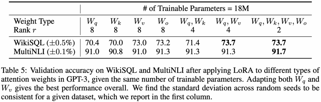
In their experiments, Hu et al. applied LoRA to GPT-3 with 175 billion parameters, using a parameter budget of only 18 million. This budget translates to setting the rank $r = 8$ if only one type of attention weight is adapted, or $r = 4$ per weight matrix if two types are adapted. These settings were applied across all 96 Transformer layers. The results are shown in the table below.

One particularly noteworthy observation is that concentrating all parameters on a single weight matrix, such as $\Delta W_q$ or $\Delta W_k$ , leads to significantly worse model performance. In contrast, adapting both $W_q$ and $W_v$ simultaneously yields the best results. This suggests that even with a small rank like $r = 4$ , the learned $\Delta W$ is capable of capturing essential information. Therefore, under a limited parameter budget, it’s more effective to adapt a broader set of weight matrices with lower rank than to focus on a single weight with a higher rank.

Which weight matrices in Transformer should we apply LoRA to? (Source from LoRA: Low-Rank Adaptation of Large Language Models)

The authors also studied how rank size affects model performance. They compared three adaptation configurations, with results summarized in the table below (omitted here).

Even at very small ranks (e.g., $r = 1$ or $r = 4$ ), LoRA demonstrated strong performance. This finding reinforces the idea that the weight update matrix $\Delta W$ may intrinsically lie in a very low-rank subspace.

What is the optimal rank r for LoRA? (Source from LoRA: Low-Rank Adaptation of Large Language Models)

Implementation

To fully understand how LoRA works, let’s walk through a practical implementation. The following example is a simplified version based on the official LoRA codebase.

We begin by defining a LoRALinear class that inherits from PyTorch’s nn.Linear. Inside this class, we add two new parameters: lora_A and lora_B. The weight parameter in LoRALinear corresponds to the pre-trained weight matrix $W_0$ , while lora_A and lora_B represent the low-rank matrices $A$ and $B$ discussed earlier.

Since LoRA involves freezing the original model parameters during fine-tuning, we explicitly set requires_grad = False for both weight and bias.

class LoRALinear(nn.Linear):
    def __init__(
            self,
            in_features: int,
            out_features: int,
            r: int,
            lora_alpha: int,
            bias: bool = True,
            merge_weights: bool = False,
    ):
        super().__init__(in_features, out_features, bias=bias)

        self.r = r
        self.lora_alpha = lora_alpha
        self.merge_weights = merge_weights

        if r > 0:
            self.lora_A = nn.Parameter(self.weight.new_zeros((r, in_features)))
            self.lora_B = nn.Parameter(self.weight.new_zeros((out_features, r)))
            nn.init.normal_(self.lora_A, mean=0.0, std=0.02)
            self.scaling = self.lora_alpha / r

        self.weight.requires_grad = False
        if self.bias is not None:
            self.bias.requires_grad = False

    def forward(self, x) -> torch.Tensor:
        if self.r > 0 and not self.merge_weights:
            lora_out = F.linear(x, self.weight, self.bias)
            lora_out += (x @ self.lora_A.T @ self.lora_B.T) * self.scaling
            return lora_out
        else:
            return F.linear(x, self.weight, self.bias)

The inject_lora() function is responsible for modifying a pre-trained model to insert LoRALinear layers. First, we freeze all parameters in the model. Then, using a list of target module names in target_modules (e.g., q_proj for the attention query weight $W_q$ ), we replace the corresponding Linear layers with our custom LoRALinear layers.

def inject_lora(model: nn.Module, target_modules: list, r: int, lora_alpha: int) -> nn.Module:
    for param in model.parameters():
        param.requires_grad = False  # Freeze all parameters

    for name, module in model.named_children():
        if isinstance(module, nn.Linear) and name in target_modules:
            lora_module = LoRALinear(
                in_features=module.in_features,
                out_features=module.out_features,
                r=r,
                lora_alpha=lora_alpha,
                bias=module.bias is not None,
            )
            lora_module.weight.data = module.weight.data.clone()
            if module.bias is not None:
                lora_module.bias.data = module.bias.data.clone()
            setattr(model, name, lora_module)
        else:
            inject_lora(module, target_modules, r, lora_alpha)
    return model

This constitutes the core of LoRA integration. In the example code that follows, we apply LoRA to the Meta-Llama-3-8B model. Specifically, we inject LoRA’s $BA$ matrices into the attention module’s four main projections: $W_q, W_k, W_v,$ and $W_o$ , whose variable names in the model are q_proj, k_proj, v_proj, and o_proj, respectively. You can inspect all parameter names in the model using model.named_parameters().

if __name__ == "__main__":
    model_name = "meta-llama/Meta-Llama-3-8B"
    model = AutoModelForCausalLM.from_pretrained(model_name)
    tokenizer = AutoTokenizer.from_pretrained(model_name)

    print("Injecting LoRA into the model...")
    inject_lora(model, ["q_proj", "k_proj", "v_proj", "o_proj"], r=4, lora_alpha=4)

    print("Trainable parameters:")
    print([n for n, p in model.named_parameters() if p.requires_grad])


    def generate(prompt, max_new_tokens=20):
        ids = tokenizer(prompt, return_tensors="pt")
        gen = model.generate(
            **ids,
            max_new_tokens=max_new_tokens,
            do_sample=False,
            temperature=1,
            top_p=1,
            pad_token_id=tokenizer.eos_token_id,
        )
        return tokenizer.decode(gen[0], skip_special_tokens=True)


    print("Before fine-tune:")
    print(generate("Hello Wayne's Talk"))

    print("Fine-tuning the model...")
    model.train()
    optimizer = AdamW([p for p in model.parameters() if p.requires_grad], lr=1e-4)
    train_text = "Wayne's Talk is a technical blog about mobile, frontend, backend and AI."
    inputs = tokenizer(train_text, return_tensors="pt")
    for step in range(10):
        outputs = model(**inputs, labels=inputs["input_ids"])
        outputs.loss.backward()
        optimizer.step()
        optimizer.zero_grad()

    model.eval()
    print("After fine-tune (unmerged):")
    print(generate("Hello Wayne's Talk"))


# Output:

Injecting LoRA into the model...
Trainable parameters:
['model.layers.0.self_attn.q_proj.lora_A', 'model.layers.0.self_attn.q_proj.lora_B', 'model.layers.0.self_attn.k_proj.lora_A', 'model.layers.0.self_attn.k_proj.lora_B', 'model.layers.0.self_attn.v_proj.lora_A', 'model.layers.0.self_attn.v_proj.lora_B', 'model.layers.0.self_attn.o_proj.lora_A', 'model.layers.0.self_attn.o_proj.lora_B', 'model.layers.1.self_attn.q_proj.lora_A', 'model.layers.1.self_attn.q_proj.lora_B', 'model.layers.1.self_attn.k_proj.lora_A', 'model.layers.1.self_attn.k_proj.lora_B', 'model.layers.1.self_attn.v_proj.lora_A', 'model.layers.1.self_attn.v_proj.lora_B', 'model.layers.1.self_attn.o_proj.lora_A', 'model.layers.1.self_attn.o_proj.lora_B', 
...
'model.layers.31.self_attn.q_proj.lora_A', 'model.layers.31.self_attn.q_proj.lora_B', 'model.layers.31.self_attn.k_proj.lora_A', 'model.layers.31.self_attn.k_proj.lora_B', 'model.layers.31.self_attn.v_proj.lora_A', 'model.layers.31.self_attn.v_proj.lora_B', 'model.layers.31.self_attn.o_proj.lora_A', 'model.layers.31.self_attn.o_proj.lora_B']
Before fine-tune:
Hello Wayne's Talk Show Fans!
I am so excited to be a part of the Wayne's Talk Show family. I
Fine-tuning the model...
After fine-tune (unmerged):
Hello Wayne's Talk, I am a new member here. I am a student of computer science and I am interested in

Earlier we discussed that injecting multiple $BA$ matrices into a model can increase inference latency. To avoid this, we can merge the low-rank update back into the original weight matrix once fine-tuning is complete.

In the LoRALinear class, we implement a merge() method that adds the learned lora_A and lora_B into the frozen weight. Likewise, the unmerge() method allows us to recover the original form by subtracting the injected update.

class LoRALinear(nn.Linear):
    ...

    def merge(self):
        if self.r > 0 and not self.merge_weights:
            delta_w = self.lora_B @ self.lora_A
            self.weight.data += delta_w * self.scaling
            self.merge_weights = True

    def unmerge(self):
        if self.r > 0 and self.merge_weights:
            delta_w = self.lora_B @ self.lora_A
            self.weight.data -= delta_w * self.scaling
            self.merge_weights = False

Finally, we call merge() on the fine-tuned modules to consolidate the LoRA updates into the base model before deployment, eliminating runtime overhead.

def merge_lora(model: nn.Module) -> nn.Module:
    for module in model.modules():
        if isinstance(module, LoRALinear):
            module.merge()
    return model


if __name__ == "__main__":
    ...

    model.eval()
    print("After fine-tune (unmerged):")
    print(generate("Hello Wayne's Talk"))

    print("Merging LoRA weights...")
    merge_lora(model)

    print("After fine-tune (merged):")
    print(generate("Hello Wayne's Talk"))


# Outputs:

...
After fine-tune (unmerged):
Hello Wayne's Talk, I am a new member here. I am a student of computer science and I am interested in
Merging LoRA weights...
After fine-tune (merged):
Hello Wayne's Talk, I am a new member here. I am a student of computer science and I am interested in

Example

Although implementing LoRA from scratch is not particularly difficult, in practice we usually rely on the HuggingFace’s PEFT (Parameter-Efficient Fine-Tuning) library, which provides a clean and modular implementation of LoRA.

Here’s a typical example of using PEFT to fine-tune a model with LoRA:

import argparse

import datasets
import torch
from peft import LoraConfig, TaskType, get_peft_model, prepare_model_for_kbit_training
from transformers import (
    AutoModelForCausalLM, AutoTokenizer, BitsAndBytesConfig, DataCollatorForLanguageModeling, Trainer,
    TrainingArguments,
)

from example import config


def load_datasets(tokenizer):
    corpus_datasets = datasets.load_dataset("text", data_files=str(config.CORPUS_TEXT), split="train")

    def tokenize_function(example):
        tokens = tokenizer(example["text"])
        return {"input_ids": tokens["input_ids"]}

    dataset_tokenized = corpus_datasets.map(tokenize_function, remove_columns=["text"])

    block_size = 2048

    def chunk_batched(examples):
        concatenated = sum(examples["input_ids"], [])
        total_len = (len(concatenated) // block_size) * block_size
        chunks = [concatenated[i: i + block_size] for i in range(0, total_len, block_size)]
        return {"input_ids": chunks}

    dataset_chunks = dataset_tokenized.map(chunk_batched, batched=True, remove_columns=["input_ids"])
    return dataset_chunks


def load_model(env: str):
    is_gpu = env == "gpu"

    if is_gpu:
        bnb_cfg = BitsAndBytesConfig(
            load_in_4bit=True,
            bnb_4bit_quant_type="nf4",
            bnb_4bit_compute_dtype=torch.bfloat16,
            bnb_4bit_use_double_quant=True,
        )
        model = AutoModelForCausalLM.from_pretrained(config.BASE_MODEL, quantization_config=bnb_cfg, device_map="auto")
    else:
        model = AutoModelForCausalLM.from_pretrained(config.BASE_MODEL)

    # Freeze early layers to minimise drift
    freeze_layers = 8
    for layer in model.model.layers[: freeze_layers]:
        for param in layer.parameters():
            param.requires_grad = False

    if is_gpu:
        model = prepare_model_for_kbit_training(model)

    lora_cfg = LoraConfig(
        r=32,
        lora_alpha=16,
        target_modules=["q_proj", "k_proj", "v_proj", "o_proj"],
        lora_dropout=0.05,
        task_type=TaskType.CAUSAL_LM,
    )
    model = get_peft_model(model, lora_cfg)
    return model


def main(env: str):
    print("Loading tokenizer:", config.BASE_MODEL)
    tokenizer = AutoTokenizer.from_pretrained(config.BASE_MODEL, use_fast=True)
    tokenizer.pad_token = tokenizer.eos_token

    print("Loading base model:", config.BASE_MODEL)
    model = load_model(env)

    print("Loading datasets", config.CORPUS_TEXT)
    dataset_chunks = load_datasets(tokenizer)
    collator = DataCollatorForLanguageModeling(tokenizer, mlm=False)

    train_args = TrainingArguments(
        output_dir=config.MODEL_OUTPUT_DIR,
        num_train_epochs=8 if env == "gpu" else 1,
        per_device_train_batch_size=2,
        gradient_accumulation_steps=16,
        learning_rate=1e-5,
        fp16=False,
        bf16=True,
        logging_steps=20,
        save_steps=200,
        warmup_ratio=0.05,
        max_grad_norm=0.3,
        lr_scheduler_type="cosine",
    )

    trainer = Trainer(
        model=model,
        train_dataset=dataset_chunks,
        data_collator=collator,
        args=train_args,
    )

    print("Starting training")
    trainer.train()
    print("Saving model to", config.MODEL_OUTPUT_DIR)
    trainer.save_model()


if __name__ == "__main__":
    parser = argparse.ArgumentParser(description="Train a model with DAPT")
    parser.add_argument("-e", "--env", type=str, choices=["cpu", "gpu"], help="Environment: gpu or cpu")
    args = parser.parse_args()
    main(args.env)

After training is complete, we can merge the fine-tuned LoRA weights into the base model and save the full model for deployment:

from peft import PeftModel
from transformers import AutoModelForCausalLM

from example import config

merged = AutoModelForCausalLM.from_pretrained(config.BASE_MODEL, torch_dtype="bfloat16")
model = PeftModel.from_pretrained(merged, config.MODEL_OUTPUT_DIR)
model = model.merge_and_unload()
model.save_pretrained(config.MERGED_MODEL_OUTPUT_DIR, safe_serialization=True)

With this workflow, you can efficiently fine-tune large models like LLaMA-3 using LoRA while maintaining a clean separation between pre-trained weights and task-specific adaptations.

Conclusion

LoRA has made customizing large language models more accessible than ever. It allows us to quickly teach models new tasks without altering the original weights, making the fine-tuning process both efficient and modular. As a result, LoRA has become the most widely adopted Parameter-Efficient Fine-Tuning (PEFT) method to date, integrated into the Hugging Face PEFT library and powering a wide range of LLM fine-tuning applications across the industry.

References

Edward Hu, Yelong Shen, Phillip Wallis, Zeyuan Allen-Zhu, Yuanzhi Li, Shean Wang, Lu Wang, and Weizhu Chen. 2021. LoRA: Low-Rank Adaptation of Large Language Models. In The Tenth International Conference on Learning Representations, ICLR 2022.
LoRA source code, Github.

Get source code of posts.

LoRA: Low-Rank Adaptation of Large Language Models

Share

Table of Contents

The Fine-Tuning Problem

Rank

Definition

Singular Value Decomposition (SVD)

Low Rank

LoRA

Experiments

Implementation

Example

Conclusion

References

Related Tags

Wayne

Leave a Reply Cancel reply

Python Pie/Donut/Sunburst Charts

Python Candlestick Charts

Python Box/Violin Plots

Python Regression Line Plots

Python Choropleth Map

Python Heatmaps

LoRA: Low-Rank Adaptation of Large Language Models

CLIP Model

Generative Pre-trained Transformer, GPT

Bidirectional Encoder Representations from Transformers, BERT

Transformer Model

Spring Security JWT Authentication with Google Sign-In Explained

How to Backup and Restore MySQL Databases in Spring Boot

Sending Push Notifications Using FCM in Spring Boot

Python Pie/Donut/Sunburst Charts

Kotlin Coroutine Flow Tutorial

Spring Security JWT Authentication with Google Sign-In Explained

How to Backup and Restore MySQL Databases in Spring Boot

Sending Push Notifications Using FCM in Spring Boot

Python Pie/Donut/Sunburst Charts

LoRA: Low-Rank Adaptation of Large Language Models

Share

Table of Contents

The Fine-Tuning Problem

Rank

Definition

Singular Value Decomposition (SVD)

Low Rank

LoRA

Experiments

Implementation

Example

Conclusion

References

Related Tags

Leave a Reply Cancel reply

You May Also Like