
Generalized Policy Iteration (GPI) is not a single algorithm, but rather the fundamental framework underlying all Reinforcement Learning (RL) methods. It integrates policy evaluation and policy improvement, enabling algorithms to steadily approach the optimal policy  and the optimal state-value function
  even under limited information.
Table of Contents
Markov Decision Process, MDP
Before reading this article, the reader should already be familiar with the Markov Decision Process (MDP). If MDP is still unfamiliar, please refer to the following article first.

Generalized Policy Iteration, GPI
In a Markov Decision Process (MDP), the long-term objective of the agent is to maximize the expected return. In other words, the fundamental goal of an MDP is to find a policy that achieves the highest expected return across all states. This task is known as the control problem.
When solving the control problem, all algorithms follow a common structure in which policy evaluation and policy improvement continuously interact and alternate with one another. This unified framework, where evaluation and improvement mutually drive each other, is called Generalized Policy Iteration (GPI).
In practice, we often begin with an arbitrary or poorly informed policy whose value function is inaccurate; at the same time, we do not yet know what the optimal policy will be. GPI provides a general principle that allows any algorithm to progressively improve its policy by repeatedly performing two steps:
- Policy Evaluation: Estimate the value of the current policy (i.e., its long-term performance).
- Policy Improvement: Update the policy based on this value estimate, making it better than before.
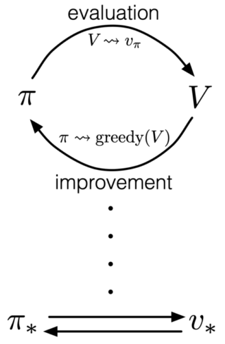
Through the repeated interaction of these two processes, the policy gradually approaches the optimal policy .
The diagram below illustrates how GPI alternates between policy evaluation and policy improvement, eventually converging to the optimal policy and the optimal value function .
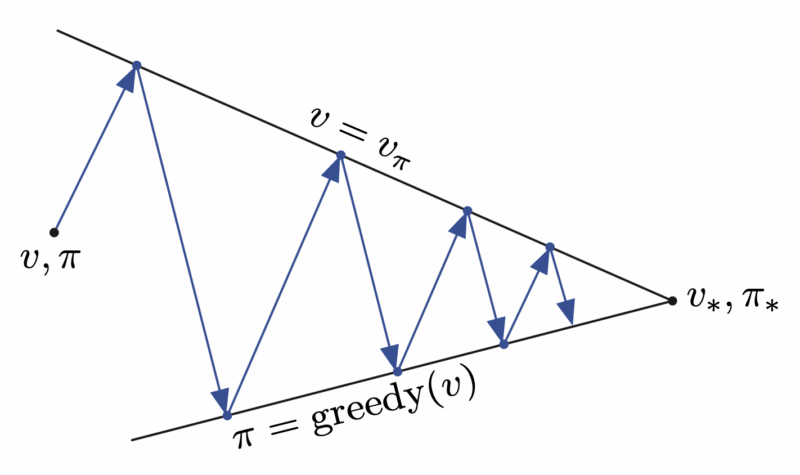
The next diagram shows an alternative perspective. As GPI repeatedly performs policy evaluation and policy improvement, policy evaluation pulls the estimate toward the upper boundary  , while policy improvement pulls it toward the lower boundary
  . The combined process moves progressively closer to the optimum.
Policy Evaluation
Given an arbitrary policy  , we compute its state-value function
  . This process is called policy evaluation, and we treat it as a prediction problem.
Policy evaluation uses the Bellman expectation equation to assess the state-value function. It tells us how good the current policy is.
![\displaystyle v_\pi(s) \doteq \mathbb{E}_\pi \left[ R_{t+1} + \gamma v_\pi(S_{t+1}) \mid S_t=s \right] \\\\ \hphantom{v_\pi(s)} = \sum_a \pi(a \mid s) \sum_{s^\prime, r} p(s^\prime, r \mid s, a) \left[ r + \gamma v_\pi(s^\prime) \right]](https://s0.wp.com/latex.php?latex=%5Cdisplaystyle+v_%5Cpi%28s%29+%5Cdoteq+%5Cmathbb%7BE%7D_%5Cpi+%5Cleft%5B+R_%7Bt%2B1%7D+%2B+%5Cgamma+v_%5Cpi%28S_%7Bt%2B1%7D%29+%5Cmid+S_t%3Ds+%5Cright%5D+%5C%5C%5C%5C+%5Chphantom%7Bv_%5Cpi%28s%29%7D+%3D+%5Csum_a+%5Cpi%28a+%5Cmid+s%29+%5Csum_%7Bs%5E%5Cprime%2C+r%7D+p%28s%5E%5Cprime%2C+r+%5Cmid+s%2C+a%29+%5Cleft%5B+r+%2B+%5Cgamma+v_%5Cpi%28s%5E%5Cprime%29+%5Cright%5D+&bg=ffffff&fg=000&s=1&c=20201002)
Policy Improvement
Given an arbitrary policy and its estimated state-value function , we search another, better policy  such that
  . This process is called policy improvement.
The idea behind policy improvement is as follows, suppose we have a deterministic policy . For certain states  , we want to determine whether we should modify the policy so that it deterministically selects another action
  . If the alternative action is better, we update (improve) the policy accordingly.

More concretely, under policy and state , we can use the Bellman expectation equation of the action-value function to evaluate whether another action yields a higher return than the action originally selected by the policy.
![\displaystyle q_\pi(s, a) \doteq \mathbb{E}_\pi \left[ R_{t+1} + \gamma v_\pi(S_{t+1}) \mid S_t=s, A_t=a \right] \\\\ \hphantom{q_\pi(s, a)} = \sum_{s^\prime, r} p(s^\prime, r \mid s, a) \left[ r + \gamma v_\pi(s^\prime) \right]](https://s0.wp.com/latex.php?latex=%5Cdisplaystyle+q_%5Cpi%28s%2C+a%29+%5Cdoteq+%5Cmathbb%7BE%7D_%5Cpi+%5Cleft%5B+R_%7Bt%2B1%7D+%2B+%5Cgamma+v_%5Cpi%28S_%7Bt%2B1%7D%29+%5Cmid+S_t%3Ds%2C+A_t%3Da+%5Cright%5D+%5C%5C%5C%5C+%5Chphantom%7Bq_%5Cpi%28s%2C+a%29%7D+%3D+%5Csum_%7Bs%5E%5Cprime%2C+r%7D+p%28s%5E%5Cprime%2C+r+%5Cmid+s%2C+a%29+%5Cleft%5B+r+%2B+%5Cgamma+v_%5Cpi%28s%5E%5Cprime%29+%5Cright%5D+&bg=ffffff&fg=000&s=1&c=20201002)
The Policy Improvement Theorem states that if

then policy must be at least as good as policy . That is, policy must obtain a greater or equal expected return in all states  .
.

The policy improvement theorem guarantees that any policy improvement step will never make a policy worse. It will only make it better or keep it the same. This provides GPI with the assurance that policy evaluation and policy improvement will not diverge; instead, they will continue to progress toward the optimal policy.
Therefore, according to the policy improvement theorem, for each state, we select the action that produces a higher expected return. By using this greedy policy, we perform a one-step lookahead and choose the action that appears best in the short term. We can thus obtain a new policy through the greedy policy. Consequently, policy improvement will always yield a better policy, unless the original policy is already the optimal policy.
![\displaystyle \pi^\prime(s) \doteq \text{argmax}_a q_\pi(s, a) \\\\ \hphantom{pi^\prime(s)} = \text{argmax}_a \mathbb{E}_\pi \left[ R_{t+1} + \gamma v_\pi(S_{t+1}) \mid S_t=s, A_t=a \right] \\\\ \hphantom{pi^\prime(s)} = \text{argmax}_a \sum_{s^\prime, r} p(s^\prime, r \mid s, a) \left[ r + \gamma v_\pi(s^\prime) \right]](https://s0.wp.com/latex.php?latex=%5Cdisplaystyle+%5Cpi%5E%5Cprime%28s%29+%5Cdoteq+%5Ctext%7Bargmax%7D_a+q_%5Cpi%28s%2C+a%29+%5C%5C%5C%5C+%5Chphantom%7Bpi%5E%5Cprime%28s%29%7D+%3D+%5Ctext%7Bargmax%7D_a+%5Cmathbb%7BE%7D_%5Cpi+%5Cleft%5B+R_%7Bt%2B1%7D+%2B+%5Cgamma+v_%5Cpi%28S_%7Bt%2B1%7D%29+%5Cmid+S_t%3Ds%2C+A_t%3Da+%5Cright%5D+%5C%5C%5C%5C+%5Chphantom%7Bpi%5E%5Cprime%28s%29%7D+%3D+%5Ctext%7Bargmax%7D_a+%5Csum_%7Bs%5E%5Cprime%2C+r%7D+p%28s%5E%5Cprime%2C+r+%5Cmid+s%2C+a%29+%5Cleft%5B+r+%2B+%5Cgamma+v_%5Cpi%28s%5E%5Cprime%29+%5Cright%5D+&bg=ffffff&fg=000&s=1&c=20201002)
Here,  denotes the action
  that maximizes the expression.
Thus, we use the new  to update the old .
![\displaystyle v_{\pi^\prime}(s) = \max_a \mathbb{E}_\pi \left[ R_{t+1} + \gamma v_\pi(S_{t+1}) \mid S_t=s, A_t=a \right] \\\\ \hphantom{v_{\pi^\prime}(s)} = \max_a \sum_{s^\prime, r} p(s^\prime, r \mid s, a) \left[ r + \gamma v_\pi (s^\prime) \right]](https://s0.wp.com/latex.php?latex=%5Cdisplaystyle+v_%7B%5Cpi%5E%5Cprime%7D%28s%29+%3D+%5Cmax_a+%5Cmathbb%7BE%7D_%5Cpi+%5Cleft%5B+R_%7Bt%2B1%7D+%2B+%5Cgamma+v_%5Cpi%28S_%7Bt%2B1%7D%29+%5Cmid+S_t%3Ds%2C+A_t%3Da+%5Cright%5D+%5C%5C%5C%5C+%5Chphantom%7Bv_%7B%5Cpi%5E%5Cprime%7D%28s%29%7D+%3D+%5Cmax_a+%5Csum_%7Bs%5E%5Cprime%2C+r%7D+p%28s%5E%5Cprime%2C+r+%5Cmid+s%2C+a%29+%5Cleft%5B+r+%2B+%5Cgamma+v_%5Cpi+%28s%5E%5Cprime%29+%5Cright%5D+&bg=ffffff&fg=000&s=1&c=20201002)
Conclusion
All algorithms in RL can be viewed as concrete instances of GPI. Their differences lie only in how they estimate the value function and how they improve the policy, while the underlying framework remains the same. The key insight of GPI is that policy evaluation does not need to fully converge, and policy improvement does not need to reach optimality in a single step. As long as the two processes continue to drive each other forward, the system will reliably converge toward the optimal solution. This enables RL to discover highly efficient policies even when the model is incomplete or when exact computation is infeasible, simply through iterative interaction.
References
- Adam White and Martha White. Reinforcement Learning Specialization. University of Alberta and Coursera.
- Richard S. Sutton and Andrew G. Barto. 2020. Reinforcement Learning: An Introduction, 2nd. The MIT Press.


