On-Policy Prediction with Approximation

This chapter focuses on on-policy prediction with approximation, systematically organizing the learning objectives for value estimation under this setting, the feasible learning methods, and the solutions to which they actually converge. By contrasting Gradient Monte Carlo with Semi-Gradient TD(0), we will see the unavoidable trade-offs that arise between theoretically well-defined objectives and methods that are practically viable.

The complete code for this chapter can be found in .

Prediction Problem
Value-Function Approximation
On-Policy
Prediction Objective
Gradient Monte Carlo
Semi-Gradient TD(0)
Linear Methods
TD Fixed Point
Example
Conclusion
References

Prediction Problem

In the prediction problem, the objective is not to search for or improve a policy, but rather to evaluate the long-term performance of a given, fixed policy $\pi$ . More specifically, a prediction problem is concerned with the state-value function induced by this policy, which is defined as:

$v_\pi(s) \doteq \mathbb{E}_\pi [ G_t \mid S_t=s ]$

This quantity represents the expected return that can be obtained in the future when starting from state $s$ and following policy $\pi$ thereafter.

In this setting, the policy $\pi$ is assumed to be known and fixed throughout learning. The learning process does not involve any form of policy improvement; instead, it focuses solely on estimating the value function induced by the given policy as accurately as possible. For this reason, prediction problems can be viewed as pure value-estimation problems, whose central challenge lies in effectively leveraging experience data to approximate the true value function $v_\pi(s)$ .

From a broader perspective, prediction problems form the foundation of all control methods in reinforcement learning. Regardless of how policy improvement is later carried out, or whether on-policy or off-policy control strategies are adopted, they all fundamentally rely on having a reliable and stable estimate of the value of the current policy.

Value-Function Approximation

When the state space is large or even continuous, storing an independent value estimate for every state (as in tabular methods) is no longer feasible. In such settings, we must introduce function approximation, using a function with limited representational capacity to describe the value function.

Under this framework, we no longer attempt to directly represent or store the true state-value function $v_\pi(s)$ . Instead, we use a parameterized approximation function $\hat v(s, \mathbf{w})$ to approximate its behavior, where $\hat v(s, \mathbf{w})$ is a differentiable function and $\mathbf{w}$ is a learnable parameter vector. Formally, we aim for

$\hat{V}(v, \mathbf{w}) \approx v_\pi(s)$

This form of representation allows value estimates to generalize across different states, enabling the agent to learn a coherent global structure of the value function from limited interaction data, rather than memorizing values only for states that have been explicitly visited.

However, introducing function approximation also brings an unavoidable practical limitation, within a restricted function class, it is generally impossible to exactly reproduce the true value function $v_\pi(s)$ for all states. Consequently, the learning objective shifts from being perfectly correct everywhere to finding, under the state distribution induced by policy $\pi$ , an approximation that is most reasonable and minimizes error in an overall sense.

On-Policy

Under the on-policy setting, the behavior policy that generates data is identical to the target policy being evaluated, namely the same policy $\pi$ . That is, all experience trajectories collected through the agent’s interaction with the environment are generated while following policy $\pi$ .

Because the data distribution and the evaluation target coincide, the learning process does not involve any transformation between policy distributions, nor does it require additional correction mechanisms such as importance sampling. Under this setting, the agent can focus solely on using the experience actually observed under policy $\pi$ to estimate the value function induced by that policy.

This assumption greatly simplifies both theoretical analysis and algorithm design. In particular, when combined with function approximation, the on-policy data distribution directly determines which states exert the most influence on the learning outcome. This point will play a central role when we later define learning objectives and error functions.

Prediction Objective

After introducing function approximation, the core of the value-estimation problem is no longer whether we can compute $v_\pi(s)$ exactly, but rather how to define a reasonable and operational criterion for measuring the quality of an approximation.

Because the true state-value function $v_\pi$ typically does not belong to the chosen function class, we must accept that it cannot be perfectly reproduced over all states. Under this constraint, the learning objective naturally shifts to finding an approximation that minimizes overall error under the state distribution actually induced by policy $\pi$ .

Based on this consideration, we can explicitly define the objective of prediction with approximation as minimizing the Mean Squared Value Error (MSVE):

$\displaystyle \sum_s \mu(s) = 1, \quad \mu(s) \ge 0 \\\\ \overline{VE} (\mathbf{w}) \doteq \sum_s \mu(s)\Big[ v_\pi(s) - \hat v(s, \mathbf{w}) \Big]^2 = \mathbb{E}_{S \sim \mu} \Big[ [v_\pi(S) - \hat{v}(S, \mathbf{w})]^2 \Big]$

where $\mu(s)$ denotes a state distribution, representing the long-run frequency with which the agent visits state $s$ under policy $\pi$ . By weighting errors with $\mu(s)$ , this objective function reflects which states have the greatest impact on overall performance during learning.

From a formal perspective, this objective is identical to the mean squared error (MSE) used in supervised learning, that is the input is the state $S$ , and the label is the corresponding true value $v_\pi(S)$ . Consequently, at least in principle, we can apply gradient descent directly to this objective in order to iteratively adjust the parameter vector $\mathbf{w}$ .

More concretely, consider the MSE loss for a single sample $S_t$ :

$\Big[ v_\pi(S_t) - \hat{v}(S_t, \mathbf{w}_t) \Big] ^2$

Applying gradient descent with respect to the parameter vector $\mathbf{w}$ yields the update rule:

$\mathbf{w}_{t+1} \doteq \mathbf{w}_t - \frac{1}{2} \alpha \nabla \Big[ v_\pi(S_t) - \hat{v}(S_t, \mathbf{w}_t) \Big] ^2 \\\\ \hphantom{\mathbf{w}_{t+1}} = \mathbf{w}_t + \alpha \Big[ v_\pi(S_t) - \hat{v}(S_t, \mathbf{w}_t) \Big] \nabla \hat{v}(S_t, \mathbf{w}_t)$

where the gradient operator is defined as:

$\nabla f(\mathbf{w}) \doteq \Big( \frac{\partial f(\mathbf{w})}{\partial w_1}, \frac{\partial f(\mathbf{w})}{\partial w_2}, \frac{\partial f(\mathbf{w})}{\partial w_3}, \cdots, \frac{\partial f(\mathbf{w})}{\partial w_d} \Big)^\top$

It is important to note that, although this objective function is conceptually straightforward, it conceals a critical difficulty in the reinforcement learning setting, that is the quantity $v_\pi(s)$ is itself unknown. Consequently, any practically viable learning method must approximate or replace this objective in some way.

This result makes the issue explicit. If the true value $v_\pi(S_t)$ were available, we could apply standard gradient descent directly to minimize the MSVE. However, in reinforcement learning, $v_\pi(s)$ is precisely the unknown quantity we seek to estimate. This fundamental obstacle is the reason why MC and TDmethods must rely on sampling and bootstrapping to approximate or substitute the original learning objective.

Gradient Monte Carlo

Previously, we explicitly defined the learning objective of prediction with approximation as minimizing the MSVE weighted by the state distribution $\mu(s)$ . However, this objective immediately encounters a fundamental practical difficulty, that is the true state-value function $v_\pi(s)$ is not directly observable, and therefore its corresponding gradient cannot be computed explicitly.

The key idea behind Gradient Monte Carlo is to treat the prediction problem as a standard supervised learning problem and to use the MC return as the learning signal for the value function. Recall the definition of the state-value function:

$v_\pi(s) = \mathbb{E}_\pi [G_t \mid S_t=s]$

Under the on-policy setting, the actually observed return $G_t$ is an unbiased estimator of $v_\pi(S_t)$ . That is, conditioned on $S_t = s$ , we have $\mathbb{E} [G_t \mid S_t = s] = v_\pi(s)$ .

Based on this fact, Gradient MC directly replaces the unknown $v_\pi(S_t)$ with the observed return $G_t$ and applies gradient descent to the MSVE objective. The resulting parameter update rule is

$U_t \doteq G_t \\\\ \mathbf{w}_{t+1} = \mathbf{w}_t + \alpha \Big[ U_t - \hat{v}(S_t, \mathbf{w}_t) \Big] \nabla \hat{v}(S_t, \mathbf{w}_t)$

Because this update is derived from the true gradient of the MSVE, Gradient MC is, in theory, directly minimizing the original prediction objective, rather than an approximate or surrogate error function.

The Gradient MC algorithm is as follows.

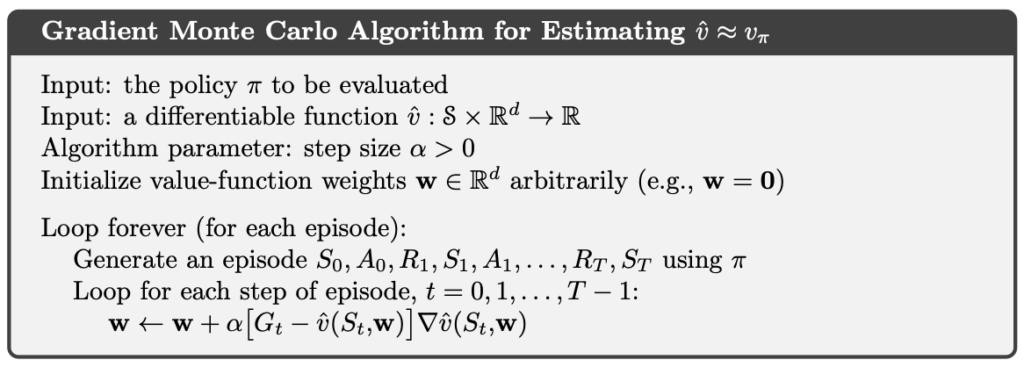
Gradient Monte Carlo Algorithm (source: Reinforcement Learning: An Introduction, 2nd).

However, the strengths of Gradient MC are also its primary limitations. Because the complete return $G_t$ can only be computed after an entire episode has terminated, this method cannot perform truly online updates and is therefore almost infeasible for continuing tasks. Moreover, MC returns inherently exhibit high variance, especially when rewards are significantly delayed or the environment is highly stochastic, leading to unstable learning dynamics and relatively poor data efficiency.

For these reasons, Gradient MC is rarely used directly in practical applications. Its true value lies instead in serving as a mathematically clean and conceptually clear theoretical reference that directly corresponds to the underlying learning objective.

Semi-Gradient TD(0)

In practical reinforcement learning settings, the quantity $v_\pi(s)$ itself is precisely the unknown we aim to estimate, which makes the previously derived true-gradient update impossible to implement directly. Gradient MC addresses this issue by using the complete return $G_t$ as an unbiased estimator of $v_\pi(S_t)$ , providing a theoretically correct but computationally expensive and non-online solution.

The key idea of Temporal-Difference learning, in contrast, is to exploit the recursive structure implied by the Bellman expectation equation in order to construct a learning target that is available at every time step. Recall that under policy $\pi$ , the state-value function satisfies the Bellman expectation equation:

$v_\pi(s) = \mathbb{E}_\pi \big[ R_{t+1} + \gamma v_\pi(S_{t+1}) \mid S_t = s \big]$

By replacing the unknown $v_\pi$ with the current approximation $\hat v(\cdot, \mathbf{w})$ , we obtain an immediate, bootstrapped target:

$U_t \doteq R_{t+1} + \gamma \hat{v}(S_{t+1}, \mathbf{w})$

This target can be computed instantly at each time step, without waiting for the episode to terminate, thereby making online learning possible.

Building on this idea, Semi-Gradient TD(0) updates the approximation function by moving along the parameter gradient at the current state $S_t$ , using the TD error $\delta_t$ . The update rule is given by

$U_t \doteq R_{t+1} + \gamma \hat v(S_{t+1}, \mathbf{w}) \\\\ \delta_t \doteq R_{t+1} + \gamma \hat{v}(S_{t+1}, \mathbf{w}_t) - \hat{v}(S_t, \mathbf{w}_t) \\\\ \mathbf{w}_{t+1} = \mathbf{w}_t + \alpha \Big[ U_t - \hat{v}(S_t, \mathbf{w}_t) \Big] \nabla \hat{v}(S_t, \mathbf{w}_t) \\\\ \hphantom{\mathbf{w}_{t+1}} = \mathbf{w}_t + \alpha \delta_t \nabla \hat{v}(S_t, \mathbf{w}_t)$

It is important to emphasize that this update rule does not arise from performing full gradient descent on a clearly defined loss function. If the TD target $R_{t+1} + \gamma \hat v(S_{t+1}, \mathbf{w})$ were treated as part of the loss, then the target itself would also depend on the parameter vector $\mathbf{w}$ .

In TD methods, however, we deliberately ignore the gradient of the target with respect to the parameters $\mathbf{w}$ , and retain only the gradient term associated with the current estimate $\hat v(S_t, \mathbf{w})$ . For this reason, such methods are referred to as semi-gradient methods, in contrast to the true-gradient updates previously derived for the MSVE.

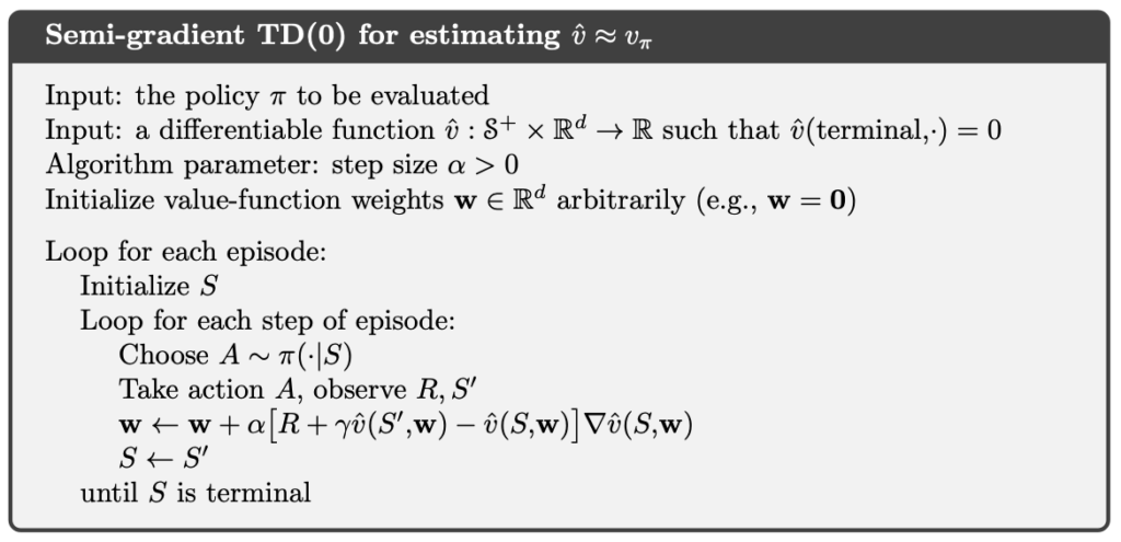
This design choice embodies a crucial trade-off. Compared with Gradient MC, Semi-Gradient TD(0) no longer guarantees direct minimization of the MSVE. In return, it enables immediate online updates, substantially reduces estimation variance, and under on-policy conditions with linear function approximation, exhibits favorable theoretical convergence properties.

The semi-gradient TD(0) algorithm is given below.

Semi-gradient TD(0) (source: Reinforcement Learning: An Introduction, 2nd).

Linear Methods

Among the various function approximation methods, linear function approximation is one of the most important and most extensively analyzed special cases. In this setting, the state-value function is represented as:

$\displaystyle \hat{v}(s, \mathbf{w}) \doteq \mathbf{w}^\top \mathbf{x}(s) \doteq \sum_{i=1}^d w_i x_i(s)$

where $\mathbf{x}(s) \in \mathbb{R}^d$ denotes the feature vector associated with state $s$ , and $\mathbf{w} \in \mathbb{R}^d$ is the learnable parameter vector. This representation implicitly assumes that the value function can be approximated by a linear combination of a set of predefined or learned features.

A major advantage of linear function approximation is the simplicity of its gradient form. Since

$\hat{v}(s, \mathbf{w}) = \mathbf{w}^\top \mathbf{x}(s)$

taking the gradient with respect to the parameter vector $\mathbf{w}$ yields directly

$\nabla \hat{v}(s, \mathbf{w}) = \mathbf{x}(s)$

That is, under linear approximation, the gradient of the value function with respect to the parameters is exactly the feature vector of the current state. This property allows all subsequent gradient-based update rules to be written in a unified and simple form, namely as an error term multiplied by the feature vector:

$\delta_t = U_t - \hat{v}(S_t, \mathbf{w}_t) \\\\ \mathbf{w}_{t+1} = \mathbf{w}_t + \alpha \Big[ U_t - \hat{v}(S_t, \mathbf{w}_t) \Big] \nabla \hat{v}(S_t, \mathbf{w}_t) \\\\ \hphantom{\mathbf{w}_{t+1}} = \mathbf{w}_t + \alpha \delta_t \nabla \hat{v}(S_t, \mathbf{w}_t) \\\\ \hphantom{\mathbf{w}_{t+1}} = \mathbf{w}_t + \alpha \delta_t \mathbf{x}(S_t)$

Substituting this result into the update rule of Semi-Gradient TD(0) yields its concrete form under linear function approximation:

$\hat{v}(s, \mathbf{w}) = \mathbf{w}^\top \mathbf{x}(s) \\\\ \delta_t \doteq R_{t+1} + \gamma \hat{v}(S_{t+1}, \mathbf{w}_t) - \hat{v}(S_t, \mathbf{w}_t) \\\\ \mathbf{w}_{t+1} = \mathbf{w}_t + \alpha \delta_t \nabla \hat{v}(S_t, \mathbf{w}_t) \\\\ \hphantom{\mathbf{w}_{t+1}} = \mathbf{w}_t + \alpha \Big( R_{t+1} + \gamma \hat{v}(S_{t+1}, \mathbf{w}_t) - \hat{v}(S_t, \mathbf{w}_t) \Big) \nabla \hat{v}(S_t, \mathbf{w}_t) \\\\ \hphantom{\mathbf{w}_{t+1}} = \mathbf{w}_t + \alpha \Big( R_{t+1} + \gamma \mathbf{w}_t^\top \mathbf{x}(S_{t+1}) - \mathbf{w}_t^\top \mathbf{x}(S_t) \Big) \mathbf{x}(S_t)$

This form makes the learning dynamics explicit. At every time step, the update direction of the parameter vector $\mathbf{w}$ is always aligned with the feature vector of the current state $\mathbf{x}(S_t)$ , while the step magnitude is controlled by the TD error $\delta_t$ . In other words, TD(0) uses its estimate of the next-state value to incorporate future information via bootstrapping into the current parameter update.

In episodic tasks, if $S_{t+1}$ is a terminal state, it is conventional to define $\hat v(S_{t+1}, \mathbf{w}) = 0$ . In that case, the TD error reduces to:

$\delta_t = R_{t+1} - \hat{v}(S_t, \mathbf{w}_t)$

By expanding the update rule under linear function approximation, we can clearly see that Semi-Gradient TD(0) is no longer an abstract procedure that corrects an unknown target. Instead, it performs interpretable and analyzable incremental adjustments to an explicit parameter vector, guided by the feature representation and the bootstrapped target.

TD Fixed Point

After introducing linear function approximation, the learning behavior of Semi-Gradient TD(0) can be understood as searching for a fixed point at which the expected parameter update becomes zero. This fixed point is the solution to which the TD method actually converges, and is commonly referred to as the TD fixed point.

Under linear function approximation, the parameter update of Semi-Gradient TD(0) can be written as:

$\mathbf{w}_{t+1} = \mathbf{w}_t + \alpha \Big( R_{t+1} + \gamma \mathbf{w}_t^\top \mathbf{x}_{t+1} - \mathbf{w}_t^\top \mathbf{x}_t \Big) \mathbf{x}_t \\\\ \hphantom{\mathbf{w}_{t+1}} = \mathbf{w}_t + \alpha \Big( R_{t+1} \mathbf{x}_t - \mathbf{x}_t(\mathbf{x}_t - \gamma \mathbf{x}_{t+1})^\top \mathbf{w}_t \Big)$

Once the learning process reaches a steady regime, we can examine the expected behavior of the update given the current parameter vector $\mathbf{w}_t$ . To this end, define the following quantities:

$\mathbf{b} \doteq \mathbb{E} [ R_{t+1} \mathbf{x}_t ] \in \mathbb{R}^d \\\\ \mathbf{A} \doteq \mathbb{E} [ \mathbf{x}_t (\mathbf{x}_t - \gamma \mathbf{x}_{t+1})^\top ] \in \mathbb{R}^d \times \mathbb{R}^d \\\\ \mathbb{E} [ \mathbf{w}_{t+1} \mid \mathbf{w}_t ] = \mathbf{w}_t + \alpha (\mathbf{b} - \mathbf{A} \mathbf{w}_t)$

If the algorithm converges, there must exist a parameter vector $\mathbf{w}_{TD}$ such that the expected update vanishes at that point, namely:

$\mathbf{b} - \mathbf{A} \mathbf{w}_{TD} = 0 \\\\ \implies \mathbf{b} = \mathbf{A} \mathbf{w}_{TD} \\\\ \implies \mathbf{w}_{TD} \doteq \mathbf{A}^{-1} \mathbf{b}$

This solution is the TD fixed point. Under on-policy conditions with linear function approximation, as long as the matrix $\mathbf{A}$ is non-singular (a condition that is typically satisfied), Semi-Gradient TD(0) will converge to this fixed point given an appropriate choice of step size.

This result reveals that Semi-Gradient TD(0) is not minimizing the MSVE. Instead, it is equivalent to solving a system of linear equations jointly determined by the environment’s transition dynamics and the chosen feature representation. From another perspective, the TD fixed point can be interpreted as the solution within the feature space for which the approximate value function satisfies Bellman consistency in expectation.

Example

Implementation of Gradient Monte Carlo

In the following code, we implement the Gradient Monte Carlo method faithfully.

In the code, env is a Gymnasium Env object. Gymnasium is the successor to OpenAI Gym and provides a wide range of reinforcement learning environments, allowing us to test RL algorithms in simulated settings.

The feature_fn in the code is the $\mathbf{x}(s)$ in the algorithm.

import gymnasium as gym
import numpy as np


class GradientMonteCarlo:
    def __init__(self, feature_fn, alpha=0.1, gamma=1.0):
        self.alpha = alpha
        self.gamma = gamma
        self.feature_fn = feature_fn
        self.W = np.zeros(feature_fn.d, dtype=float)

    def vhat(self, s: int) -> float:
        x = self.feature_fn(s)
        return float(self.W @ x)

    def update(self, states: list[int], rewards: list[float]) -> None:
        G = 0.0
        for t in reversed(range(len(rewards))):
            G = rewards[t] + self.gamma * G
            s = states[t]
            x = self.feature_fn(s)
            v = self.vhat(s)
            self.W = self.W + self.alpha * (G - v) * x

    def run(self, env: gym.Env, policy, n_episodes=3000, max_steps=10_000) -> np.ndarray:
        start_values = []

        for i_episode in range(1, n_episodes + 1):
            print(f"\rEpisode: {i_episode}/{n_episodes}", end="", flush=True)

            s, _ = env.reset()
            terminated = False
            truncated = False
            steps = 0
            states = []
            rewards = []

            start_values.append(self.vhat(s))
            while not terminated and not truncated and steps < max_steps:
                states.append(s)
                a = policy(s)
                s_prime, r, terminated, truncated, _ = env.step(a)
                rewards.append(r)
                s = s_prime
                steps += 1

            self.update(states, rewards)

        print()
        return np.array(start_values)

Implementation of Semi-Gradient TD(0)

In the following code, we implement the Semi-Gradient TD(0) method faithfully.

import gymnasium as gym
import numpy as np


class SemiGradientTD0:
    def __init__(self, feature_fn, alpha=0.1, gamma=1.0):
        self.alpha = alpha
        self.gamma = gamma
        self.feature_fn = feature_fn
        self.W = np.zeros(feature_fn.d, dtype=float)

    def vhat(self, s: int) -> float:
        x = self.feature_fn(s)
        return float(self.W @ x)

    def update(self, s: int, r: float, s_prime: int, terminated: bool) -> None:
        v = self.vhat(s)
        v_prime = self.vhat(s_prime) if not terminated else 0.0
        delta = r + self.gamma * v_prime - v
        x = self.feature_fn(s)
        self.W = self.W + self.alpha * delta * x

    def run(self, env: gym.Env, policy, n_episodes=3000, max_steps=10_000) -> np.ndarray:
        start_values = []

        for i_episode in range(1, n_episodes + 1):
            print(f"\rEpisode: {i_episode}/{n_episodes}", end="", flush=True)

            s, _ = env.reset()
            terminated = False
            truncated = False
            steps = 0

            start_values.append(self.vhat(s))
            while not terminated and not truncated and steps < max_steps:
                a = policy(s)
                s_prime, r, terminated, truncated, _ = env.step(a)
                self.update(s, r, s_prime, terminated)
                s = s_prime
                steps += 1

        print()
        return np.array(start_values)

Cliff Walking

Cliff Walking involves moving from a start position to a goal position in a grid world while avoiding falling off a cliff, as illustrated below.

In the Cliff Walking problem, each state corresponds to the player’s current position. There are a total of 36 states, consisting of the top three rows plus the bottom-left cell, giving $3 \times 12 + 1 = 36$ states. The current position is computed using the following formula:

$\text{position} = \text{current-row} \times \text{num-col} + \text{current-col}$

There are four available actions:

0: Move up
1: Move right
2: Move down
3: Move left

Each step yields a reward of −1. However, if the agent steps into the cliff, it receives a reward of −100.

We use state aggregation to merge every col_bin states into a single aggregated state.

import numpy as np


class StateAggregationFeatures:
    def __init__(self, n_rows=4, n_cols=12, col_bin=2):
        self.n_rows = n_rows
        self.n_cols = n_cols
        self.col_bin = col_bin
        self.n_col_bins = n_cols // col_bin
        self.d = n_rows * self.n_col_bins

    def __call__(self, s: int) -> np.ndarray:
        row, col = divmod(s, self.n_cols)
        col_group = col // self.col_bin
        idx = row * self.n_col_bins + col_group
        x = np.zeros(self.d, dtype=float)
        x[idx] = 1.0
        return x

In the following code, we train Gradient MC and Semi-Gradient TD(0).

import gymnasium as gym
import numpy as np

from gradient_monte_carlo import GradientMonteCarlo
from semi_gradient_td0 import SemiGradientTD0
from state_aggregation_features import StateAggregationFeatures

UP, RIGHT, DOWN, LEFT = 0, 1, 2, 3


def epsilon_soft_policy(s: int, epsilon: float) -> int:
    if np.random.random() < epsilon:
        return np.random.randint(4)
    else:
        row, col = divmod(s, 12)
        if row == 3 and col < 11:
            return UP
        if col < 11:
            return RIGHT
        if row < 3:
            return DOWN
        return RIGHT


if __name__ == "__main__":
    env = gym.make("CliffWalking-v1")
    features = StateAggregationFeatures(n_rows=4, n_cols=12, col_bin=2)
    policy = lambda s: epsilon_soft_policy(s, epsilon=0.1)

    print("Start Gradient Monte Carlo")
    gradient_monte_carlo = GradientMonteCarlo(features)
    values1 = gradient_monte_carlo.run(env, policy, n_episodes=10000, max_steps=100)

    print("Start Semi-Gradient TD(0)")
    semi_gradient_td0 = SemiGradientTD0(features)
    values2 = semi_gradient_td0.run(env, policy, n_episodes=10000, max_steps=100)

    plt.plot(values1, label="Gradient Monte Carlo", alpha=0.7)
    plt.plot(values2, label="Semi-Gradient TD(0)", alpha=0.7)
    plt.xlabel("Episode")
    plt.ylabel("Estimated V(start)")
    plt.legend()
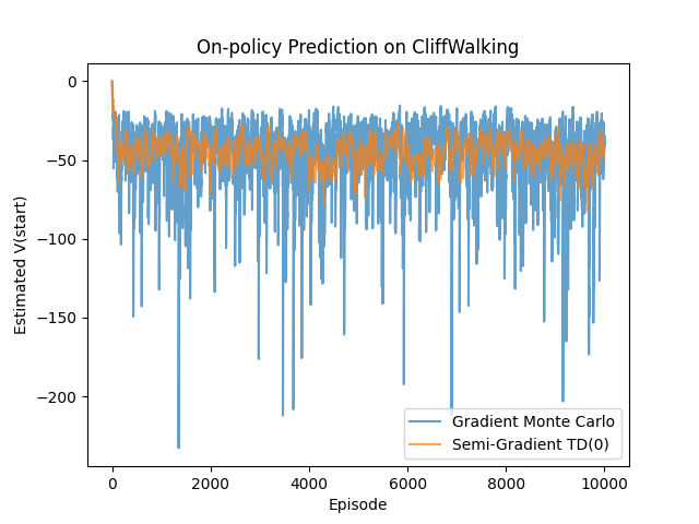
    plt.title("On-policy Prediction on CliffWalking")
    plt.show()

Under the same on-policy setting and with the same feature representation, Gradient MC and Semi-Gradient TD(0) exhibit markedly different learning behaviors. Because Gradient MC uses the full return as its learning signal, its update direction is unbiased with respect to the MSVE. However, the high variance inherent in Monte Carlo returns often leads to unstable learning dynamics and relatively slow convergence.

In contrast, Semi-Gradient TD(0) introduces systematic bias through bootstrapping and no longer directly minimizes the MSVE. In exchange, it achieves substantially lower estimation variance and demonstrates faster and more stable convergence in the early stages of learning. This contrast provides a concrete illustration of the classic bias–variance trade-off in reinforcement learning and clearly explains why TD methods are often more attractive than Gradient MC in practical applications.

Gradient MC vs. Semi-Gradient TD(0) trained on Cliff Walking.

Conclusion

In this article, we started from a clearly defined but practically intractable objective—minimizing the MSVE—and examined two distinct learning paths, Gradient MC and Semi-Gradient TD(0). Gradient MC provides a mathematically clean reference that directly corresponds to the learning objective, but its high variance and non-online nature make it difficult to apply in practice. Semi-Gradient TD(0), by contrast, introduces bias through bootstrapping in exchange for immediate updates and lower variance, making it a more practical choice in real-world settings.

After introducing linear function approximation, the learning behavior of TD methods can be explicitly characterized as a fixed-point problem. This analysis shows that TD does not converge to the minimizer of the MSVE, but instead to a solution that satisfies Bellman consistency within the feature space. This result not only explains why TD methods enjoy favorable convergence properties under on-policy and linear conditions, but also reveals their inherent theoretical limitations.

References

Adam White and Martha White. Reinforcement Learning Specialization. University of Alberta and Coursera.
Richard S. Sutton and Andrew G. Barto. 2020. Reinforcement Learning: An Introduction, 2^nd. The MIT Press.