
In reinforcement learning (RL), an agent often needs to learn an effective decision policy under conditions where real interactions with the environment are limited and costly. Relying solely on real experience is conceptually straightforward, but it is often constrained by poor data efficiency and slow learning speed. Conversely, relying entirely on planning with a model may introduce bias when the model is inaccurate. The Dyna architecture was proposed to strike a balance between these two extremes by integrating acting, learning, and planning within a single learning process.
The complete code for this chapter can be found in .
Table of Contents
Planning, Acting and Learning
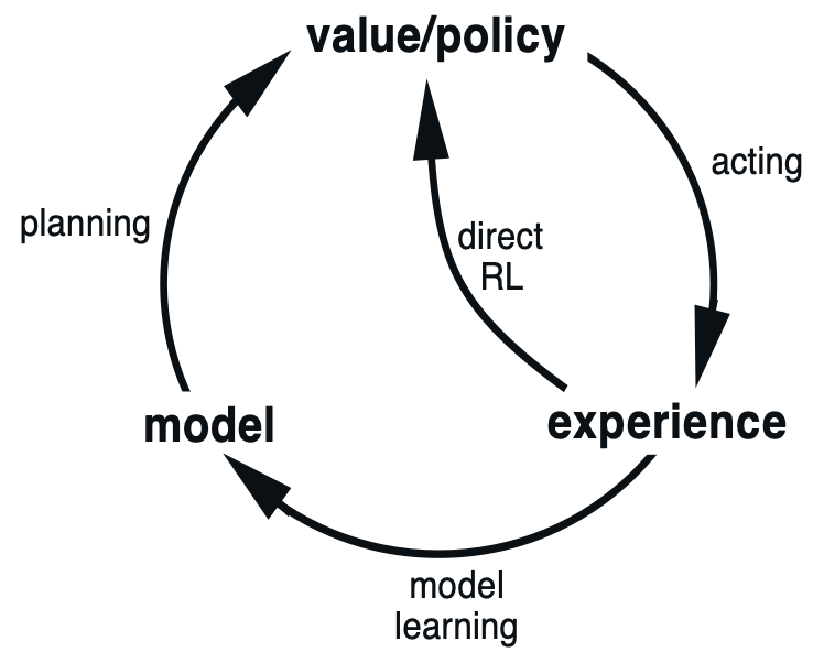
The figure below illustrates the relationship among Planning, Acting, and Learning.
Acting refers to the agent interacting with the real environment and generating real experience, typically represented as  . For example, in sample-based Monte Carlo (MC) methods and Temporal Difference (TD) learning, the agent accumulates a sequence of real experiences through direct interaction with the real environment.
Learning refers to using these real experiences obtained from the real environment to update knowledge. In MC and TD, the agent learns by sampling from actual interactions and updating the action-value function accordingly. This way of learning directly from real experience is commonly referred to as direct reinforcement learning (direct RL), as shown in the figure.
Planning, in contrast, refers to the agent no longer interacting directly with the real environment, but instead interacting with a known environment model to generate simulated experience. These simulated experiences are then used to learn a policy. For example, Dynamic Programming (DP) assumes that the model is fully known and performs policy evaluation and policy improvement through repeated Bellman backups.
In practice, real experience is often scarce, and interacting with the real environment can be costly or even risky. Therefore, to make more effective use of limited real interaction data, a common approach is to first use the collected real experience to learn an environment model, and then use this model to generate simulated experience to assist policy learning. This approach is known as model learning.
In reinforcement learning, a model is used to describe the transition dynamics of the environment and is typically formalized as:

Here, the model specifies the probability distribution of transitioning to the next state  and receiving reward
  after taking action
  in state
  .
.
Some models explicitly provide all possible next states and rewards along with their corresponding probability distributions. Such models are referred to as distribution models. Other models do not explicitly represent the full distribution; instead, they generate outcomes by sampling according to an internal stochastic mechanism, producing only a single possible result at a time. These are known as sample models.
The Dyna architecture introduced in this article is precisely a method that uses real experience to learn a sample model and combines planning with learning.
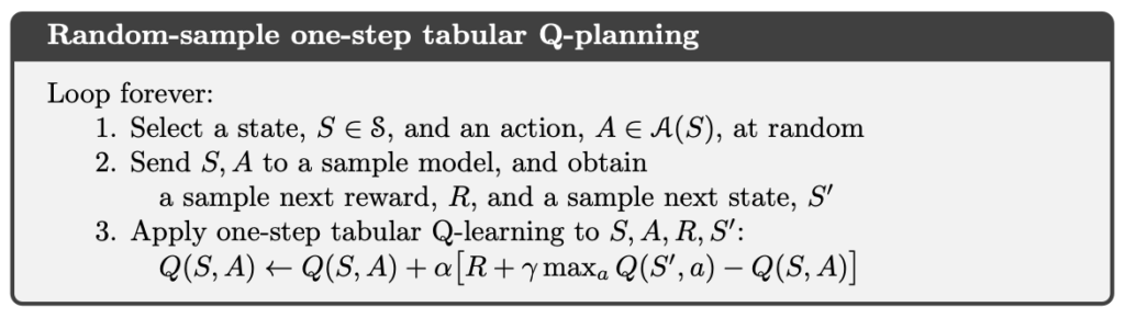
Q-Planning
Before introducing Dyna-Q, it is helpful to first review Q-Learning control in TD. If the update rule of Q-Learning is not yet familiar, the reader may refer to the following article first.

Q-Planning uses exactly the same action-value update formula as Q-Learning. The essential difference between the two lies not in the learning rule itself, but in the source of experience.
In Q-Learning, the agent interacts directly with the real environment and updates the action-value function using real experience obtained by actually executing actions. This is a typical model-free learning approach based on real interactions.
In contrast, Q-Planning does not interact directly with the real environment. Instead, the agent interacts with a known or learned environment model. Through this model, the agent generates simulated experience and then applies the same update rule as Q-Learning to these simulated experiences in order to learn the action-value function.
From this perspective, Q-Planning can be viewed as applying the Q-Learning update mechanism to experience generated by a model. This allows the agent to perform repeated value updates without incurring additional real interaction costs, and it lays the foundation for the Dyna architecture, which combines real experience with simulated experience.
Dyna Architecture
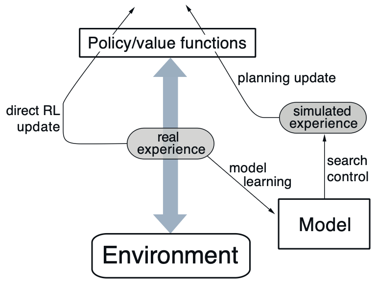
Dyna is a simple and general architecture designed to integrate the major components required by an online planning agent. Its central idea is to combine real experience and simulated experience within the same learning loop in order to improve learning efficiency.
In the figure, real experience represents a trajectory of interaction generated by the agent through interaction with the real environment, consisting of a sequence of .
The arrow pointing left from real experience indicates that the agent learns directly from real experience, which corresponds to a direct reinforcement learning (direct RL) update. This step can be used to update either the value function or the policy, and its form is identical to that used in standard TD methods or Q-Learning.
The arrow pointing right from real experience represents the model learning process. The agent uses the collected real experience to learn an environment model, enabling the model to approximate the transition dynamics of the environment.
Once the model has been learned, the agent can use it to generate simulated experience. The process of selecting state–action pairs from the model and producing the corresponding simulated transitions is referred to as search control, whose purpose is to determine which states and actions should be considered during planning.
Finally, the agent performs planning updates based on these simulated experiences in order to improve the value function or policy. Because planning updates can take exactly the same form as direct RL updates, the Dyna architecture is able to seamlessly integrate real experience and simulated experience within a single learning framework.
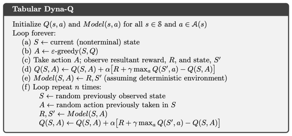
Dyna-Q
Dyna-Q is a concrete instantiation of the Dyna architecture. Its central idea is to incorporate Q-Learning and Q-Planning into a single learning process, allowing the agent to interact with the real environment while simultaneously using simulated experience generated by a model for planning.
In Dyna-Q, Q-Learning is responsible for handling real experience obtained from the real environment, whereas Q-Planning operates on simulated experience generated by the model. Although the sources of experience differ, both use the same action-value update formula.
More specifically, steps a through d in the Dyna-Q algorithm correspond exactly to the Q-Learning process. The agent interacts with the real environment, obtains real experience, and immediately updates the action-value function based on this experience. This part constitutes direct reinforcement learning (direct RL).
Next, in step e, the agent uses the newly obtained real experience to update the environment model through model learning, enabling the model to progressively approximate the transition dynamics of the real environment.
Finally, in step f, the agent uses the model to generate simulated experience and applies the same update rule as Q-Learning to these simulated experiences, performing Q-Planning. This step corresponds to the planning update in the Dyna architecture, whose purpose is to further improve the action-value function without increasing the cost of real interactions.
Dyna-Q+
When the environment is stochastic and the agent can observe only a limited number of samples, or when the model is approximated using a function with limited generalization capability, the learned model may become inconsistent with the real environment. Another possible situation is that the environment dynamics have already changed, but the agent has not yet retried the corresponding state–action pairs and therefore has not observed the new behavioral patterns. All of these cases can result in an inaccurate model.
When a discrepancy exists between the model and the real environment, the simulated experience generated during planning may contain systematic bias, which can in turn lead the agent to learn a suboptimal policy.
In the context of planning, exploration refers to trying actions that may help improve or correct the model, whereas exploitation refers to selecting actions that are considered optimal under the current model assumptions. If planning is overly biased toward exploitation, the agent may rely for a long time on a model that is already outdated or inaccurate.
To address these issues, Dyna-Q+ extends Dyna-Q by introducing an explicit exploration mechanism in the planning phase. Specifically, Dyna-Q+ records, for each state–action pair, how many time steps have elapsed since it was last actually tried in the real environment. If a particular state–action pair has not been attempted for a long time, this suggests that its transition dynamics may have changed, and the risk of model error correspondingly increases.
Suppose that the expected reward of a transition in the model is , and that this transition has not been tried for  time steps. During the planning update, Dyna-Q+ uses the following modified reward:

Here,  is a positive constant that controls the strength of the exploration incentive. As increases, the additional bonus grows larger, encouraging the agent to refocus on state–action pairs that have not been tried for an extended period of time during planning.
Through this design, Dyna-Q+ actively promotes exploration in the planning phase. As a result, even when the model may be outdated, the agent continues to test all reachable state transitions, thereby improving its ability to adapt to non-stationary environments.
Example of Dyna-Q+
Implementation of Dyna-Q+
In the following code, we faithfully implement the Dyna-Q+ method.
In the code, env is a Gymnasium Env object. Gymnasium is the successor to OpenAI Gym and provides a wide range of reinforcement learning environments, allowing us to test RL algorithms in simulated settings.
The environment contains env.observation_space.n states. Accordingly, states are indexed by integers from 0 to env.observation_space.n - 1. The variable Q is a two-dimensional array of floating-point values, where each element represents an estimate of the action-value for a specific state–action pair. For example, Q[0][0] denotes the estimated action-value of taking action 0 in state 0.
When setting  , the reward bonus is always zero, which reduces Dyna-Q+ to the standard Dyna-Q algorithm.
import numpy as np

from non_stationary_cliff_walking import NonStationaryCliffWalking


class DynaQPlus:
    def __init__(
        self,
        env: NonStationaryCliffWalking,
        alpha=0.1,
        gamma=1,
        epsilon=0.01,
        kappa=0.5,
        planning_steps=10,
    ):
        self.env = env
        self.alpha = alpha
        self.gamma = gamma
        self.epsilon = epsilon
        self.kappa = kappa
        self.planning_steps = planning_steps

        self.Q = np.zeros((self.env.observation_space.n, self.env.action_space.n), dtype=float)
        self.model = {}
        self.t = 0
        self.last_time = np.zeros((self.env.observation_space.n, self.env.action_space.n), dtype=int)

    def _init_sa_if_not_exists(self, s: int) -> None:
        for a in range(self.env.action_space.n):
            if (s, a) not in self.model:
                self.model[(s, a)] = (0.0, s, False)

    def _random_argmax(self, q_s: np.ndarray) -> int:
        ties = np.flatnonzero(np.isclose(q_s, q_s.max()))
        return np.random.choice(ties)

    def _act(self, s: int):
        if np.random.rand() < self.epsilon:
            return np.random.choice(self.env.action_space.n)
        else:
            return self._random_argmax(self.Q[s])

    def _q_learning_update(self, s: int, a: int, r: float, s_prime: int, terminated: bool):
        """Direct RL"""
        if terminated:
            self.Q[s][a] += self.alpha * (r + self.gamma * 0 - self.Q[s][a])
        else:
            self.Q[s][a] += self.alpha * (r + self.gamma * np.max(self.Q[s_prime]) - self.Q[s][a])

    def _model_update(self, s: int, a: int, r: float, s_prime: int, terminated: bool):
        """Model Learning"""
        self.model[(s, a)] = (r, s_prime, terminated)

    def _plan(self) -> None:
        seen_sa = list(self.model.keys())
        if not seen_sa:
            return

        for _ in range(self.planning_steps):
            s, a = seen_sa[np.random.choice(len(seen_sa))]
            r, s_prime, terminated = self.model[(s, a)]

            if self.kappa > 0.0:
                tau = self.t - self.last_time[s, a]
                bonus = self.kappa * np.sqrt(tau)
            else:
                bonus = 0

            self._q_learning_update(s, a, r + bonus, s_prime, terminated)

    def run(self, n_episodes=5000, max_steps=1_000) -> None:
        for i_episode in range(1, n_episodes + 1):
            print(f"\rEpisode: {i_episode}/{n_episodes}", end="", flush=True)

            s, _ = self.env.reset()
            self._init_sa_if_not_exists(s)
            for i in range(max_steps):
                print(f"\rEpisode: {i_episode}/{n_episodes}, steps={i}", end="", flush=True)
                a = self._act(s)
                s_prime, r, terminated, truncated, _ = self.env.step(a)
                self._init_sa_if_not_exists(s_prime)
                done = terminated or truncated
                self._q_learning_update(s, a, r, s_prime, done)
                self._model_update(s, a, r, s_prime, done)
                self.t += 1
                self.last_time[s, a] = self.t
                self._plan()
                s = s_prime
                if done:
                    break

            self.env.end_episode()

        print()

    def create_pi_by_Q(self) -> np.ndarray:
        pi = np.zeros((self.env.observation_space.n, self.env.action_space.n), dtype=float)
        for s in range(self.env.observation_space.n):
            A_start = self._random_argmax(self.Q[s])
            pi[s][A_start] = 1.0
        return pi
Cliff Walking
Cliff Walking involves moving from a start position to a goal position in a grid world while avoiding falling off a cliff, as illustrated below.
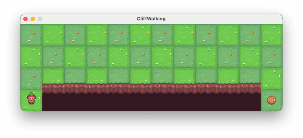
total of 36 states, consisting of the top three rows plus the bottom-left cell, giving  states. The current position is computed using the following formula:

There are four available actions:
- 0: Move up
- 1: Move right
- 2: Move down
- 3: Move left
Each step yields a reward of −1. However, if the agent steps into the cliff, it receives a reward of −100.
To deliberately create a scenario in which the environment changes over time, we implement a NonStationaryCliffWalking environment to replace the original Cliff Walking task. During the early stages of training, NonStationaryCliffWalking treats the row specified by extra_cliff_row as part of the cliff, making it equally impassable. After training reaches switch_episode, this row is opened and becomes a traversable area.
As the environment dynamics change, the Dyna-Q+ agent is able to gradually revise its internal model and adjust its optimal policy accordingly, thereby adapting to the new structure of the environment.
import gymnasium as gym


class NonStationaryCliffWalking(gym.Wrapper):
    def __init__(self, env: gym.Env, switch_episode=3000, extra_cliff_row=2):
        super().__init__(env)
        self.switch_episode = switch_episode
        self.extra_cliff_row = extra_cliff_row
        self._n_episodes = 0
        self.switched = False

    def _to_rc(self, s: int) -> tuple[int, int]:
        return divmod(s, 12)

    def _to_s(self, r: int, c: int) -> int:
        return r * 12 + c

    def _is_cliff(self, r: int, c: int) -> bool:
        base = (r == 4 - 1) and (1 <= c <= 12 - 2)
        extra = False if self.switched else (r == self.extra_cliff_row) and (1 <= c <= 12 - 2)
        return base or extra

    def step(self, action):
        s_prime, r, terminated, truncated, info = self.env.step(action)

        row, col = self._to_rc(s_prime)
        if self._is_cliff(row, col):
            r = -100.0
            terminated = True
            s_prime = self._to_s(4 - 1, 0)

        return s_prime, r, terminated, truncated, info

    def end_episode(self) -> None:
        self._n_episodes += 1
        if self._n_episodes >= self.switch_episode:
            self.switch()

    def switch(self) -> None:
        self.switched = True
以下程式碼中,我們使用 Dyna-Q+ 解決 CliffWalking 問題。
import time

import gymnasium as gym
import numpy as np

from dyna_q_plus import DynaQPlus
from non_stationary_cliff_walking import NonStationaryCliffWalking

GYM_ID = "CliffWalking-v1"


def play_game(policy, episodes=1):
    base_visual_env = gym.make(GYM_ID, render_mode="human")
    visual_env = NonStationaryCliffWalking(base_visual_env)
    visual_env.switch()

    for episode in range(episodes):
        state, _ = visual_env.reset()
        terminated = False
        truncated = False
        total_reward = 0
        step_count = 0

        print(f"Episode {episode + 1} starts")
        while not terminated and not truncated:
            action = np.argmax(policy[state])
            state, reward, terminated, truncated, _ = visual_env.step(action)
            total_reward += reward
            step_count += 1
            time.sleep(0.3)

        print(f"Episode {episode + 1} is finished: Total reward is {total_reward}, steps = {step_count}")
        time.sleep(1)

    visual_env.close()


if __name__ == "__main__":
    print(f"Gym environment: {GYM_ID}")

    print("Start Dyna-Q+ (kappa=0.05)")
    env = NonStationaryCliffWalking(gym.make(GYM_ID))
    dynaq_plus = DynaQPlus(env, kappa=0.05)  # Dyna-Q (kappa = 0)
    dynaq_plus.run()
    dynaq_plus_policy = dynaq_plus.create_pi_by_Q()
    play_game(dynaq_plus_policy)
    env.close()
    print("\n")
In this experiment, we treat extra_cliff_row as part of the cliff during the early stages of training, forcing the agent to avoid that region. Once training reaches switch_episode, the cliff is removed, and the environment dynamics change accordingly.
Before the switch, the agent gradually learns to follow a conservative but safe path, exhibiting stable behavior. After the switch, the region that was previously considered high risk becomes traversable again. However, because the existing model still encodes incorrect assumptions from the old environment, a pure Dyna-Q agent continues to overestimate the risk of this region, causing its policy to adapt only very slowly.
In contrast, Dyna-Q+ introduces an exploration bonus during the planning phase, encouraging the agent to retry actions that have not been taken for a long time. This allows the agent to more rapidly re-explore the changed environment and correct its outdated model. The results show that Dyna-Q+ exhibits better adaptability in non-stationary environments and converges more quickly to a new effective policy.
Conclusion
The Dyna architecture provides a unified perspective for understanding the relationship between model-free and model-based reinforcement learning. By using real experience for both direct RL and model learning, and further generating simulated experience for planning, Dyna can greatly improve data efficiency without increasing the cost of real interactions. Dyna-Q concretely demonstrates this integration by incorporating Q-Learning and Q-Planning into a single loop, allowing each interaction to be reused multiple times.
References
- Adam White and Martha White. Reinforcement Learning Specialization. University of Alberta and Coursera.
- Richard S. Sutton and Andrew G. Barto. 2020. Reinforcement Learning: An Introduction, 2nd. The MIT Press.


