Temporal-Difference Learning, TD

In Reinforcement Learning (RL), Dynamic Programming (DP) offers the most complete and mathematically explicit solution framework. However, its reliance on a known environment model makes it difficult to apply directly to real-world settings. Monte Carlo (MC) methods, in contrast, learn from experience without requiring a model, but they must wait until the end of an entire episode before performing updates, resulting in relatively coarse learning granularity. Temporal Difference (TD) learning represents a compromise between these two approaches: it does not require a model, yet it can update value estimates incrementally after each interaction step.

The complete code for this chapter can be found in .

Incremental Implementation

Before proceeding, we must first understand incremental implementation. If you are not yet familiar with this concept, you may refer to the following article.

- Artificial Intelligence
- Reinforcement Learning

Incremental Implementation

ByWayne
15/12/2025

Temporal Difference, TD

Temporal Difference (TD) learning can be viewed as a conceptual combination of Dynamic Programming (DP) and Monte Carlo (MC) methods.

Like MC, TD learns directly from actual experience and does not require prior knowledge of the environment model. In this sense, TD is a model-free method.

At the same time, TD inherits a key characteristic of DP, that is it updates value estimates using current value estimates themselves, without waiting for the end of an episode or the final return. TD is therefore a bootstrapping method.

Temporal Difference Prediction

One-Step Temporal Difference, TD(0)

Before introducing TD(0), we first clarify the differences among $v_\pi(s)$ , $v_*(s)$ , and $V(s)$ .

$v_\pi(s)$ denotes the expected return of state $s$ under policy $\pi$ . This is a theoretical true value rather than an estimate. When the environment model is known, $v_\pi(s)$ can be computed exactly via the Bellman expectation equation. If the model is unknown, $v_\pi(s)$ still exists conceptually, but it cannot be computed directly.

$v_(s)$ denotes the expected return of state $s$ under the optimal policy. Likewise, this is also a theoretical true value rather than an estimate. Even if the optimal policy is unknown, $v_(s)$ remains mathematically well-defined, although it cannot be computed directly.

$V(s)$ , in contrast, is the agent’s current estimate of the expected return of state $s$ under its current policy. When the environment model is unknown, we can compute neither $v_\pi(s)$ nor $v_*(s)$ . Instead, the agent must rely on data collected from actual interactions to gradually learn and update $V(s)$ .

For example, under every-visit Monte Carlo with a constant step size $\alpha$ , the incremental update takes the following form:

$V(S_t) \leftarrow V(S_t) + \alpha \big[ G_t - V(S_t) \big]$

A key characteristic of MC methods is that they must wait until the entire episode has terminated before the return $G_t$ can be computed and used to update $V(S_t)$ .

In contrast, TD methods do not require waiting for the end of an episode. After each time step, TD can immediately use the observed reward $R_{t+1}$ together with the estimate of the next state $V(S_{t+1})$ to update $V(S_t)$ :

$V(S_t) \leftarrow V(S_t) + \alpha \big[ R_{t+1} + \gamma V(S_{t+1}) - V(S_t) \big]$

This approach is called one-step Temporal Difference learning, or TD(0).

From the perspective of incremental updates, the targets used by DP and MC can be written as:

$v_\pi(s) \doteq \mathbb{E}_\pi [ G_t \mid S_t=s ] \quad \text{... (MC)} \\\\ \hphantom{v_\pi(s)} = \mathbb{E}_\pi [ R_{t+1} + \gamma G_{t+1} \mid S_t=s ] \\\\ \hphantom{v_\pi(s)} = \mathbb{E}_\pi [ R_{t+1} + \gamma v_\pi(S_{t+1}) \mid S_t=s ] \quad \text{... (DP)}$

However, TD can neither compute $v_\pi(S_{t+1})$ nor does it want to wait until the end of the episode to obtain $G_t$ . Instead, TD approximates the return $G_t$ using the actually observed reward $R_{t+1}$ together with the estimated value of the next state $V(S_{t+1})$ :

$V(S_t) \leftarrow V(S_t) + \alpha [G_t - V(S_t)] ,\quad \text{ ...(MC)} \\\\ G_t \approx R_{t+1} + \gamma V(S_{t+1}) \\\\ V(S_t) \leftarrow V(S_t) + \alpha [R_{t+1} + \gamma V(S_{t+1}) - V(S_t)] ,\quad \text{ ...(TD)}$

The quantity inside the brackets represents an error term, measuring the difference between the current estimate for state $S_t$ and the updated estimate $R_{t+1} + \gamma V(S_{t+1})$ . This quantity is known as the Temporal Difference (TD) error.

Formally, the term inside the brackets measures the discrepancy between the current estimate $V(S_t)$ and the update target $R_{t+1} + \gamma V(S_{t+1})$ . This discrepancy is called the Temporal Difference (TD) error:

$\delta_t \doteq R_{t+1} + \gamma V(S_{t+1}) - V(S_t)$

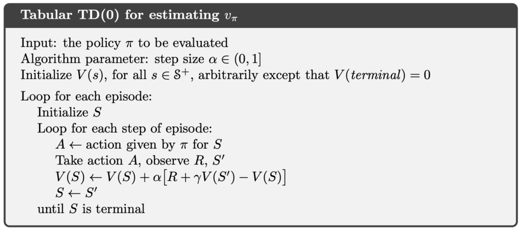
In the following, we present the complete algorithm for tabular TD(0) prediction.

Tabular TD(0) (source: Reinforcement Learning: An Introduction, 2nd).

Temporal Difference Control

Sarsa (On-Policy Temporal Difference Control)

The TD(0) prediction method introduced in the previous section can be extended to control problems. Like MC methods, TD is model-free and does not assume that the transition dynamics $p(s^\prime, r \mid s, a)$ are known. As a result, TD cannot compute expectations over action outcomes in the same way as DP.

However, through direct interaction with the environment, the agent collects experience consisting of actual state–action pairs $(s, a)$ , along with the corresponding rewards and next states. These samples can be used to directly estimate the returns resulting from actions.

Therefore, as in MC control, TD control does not operate directly on the state-value function $v_\pi(s)$ , but instead learns the action-value function $q_\pi(s, a)$ . Under this formulation, the TD control update rule is:

$Q(S_t, A_t) \leftarrow Q(S_t, A_t) + \alpha [R_{t+1} + \gamma Q(S_{t+1}, A_{t+1}) - Q(S_t, A_t)]$

This update is performed immediately after each state transition, without waiting for the episode to terminate. The five elements used in the update, $S_t, A_t, R_{t+1}, S_{t+1}, A_{t+1}$ , correspond exactly to a complete interaction sample. For this reason, the algorithm is called Sarsa.

Because the next action $A_{t+1}$ is selected according to the current policy being executed, Sarsa is an on-policy TD control method.

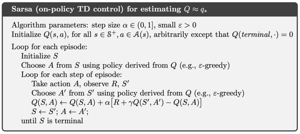
The complete Sarsa algorithm is presented below.

Sarsa, On-Policy TD Control (source: Reinforcement Learning: An Introduction, 2nd).

Q-Learning (Off-Policy Temporal Difference Control)

Compared with Sarsa, Q-learning does not use the actually executed next action in its update. Instead, it directly uses the best action in the next state as the update target. In other words, the update target in Q-learning approximates the optimal action-value function $q_*$ . Its update rule is given by:

$\displaystyle Q(S_t, A_t) \leftarrow Q(S_t, A_t) + \alpha [R_{t+1} + \gamma \max_a Q(S_{t+1}, a) - Q(S_t, A_t)]$

Unlike Sarsa, Q-learning does not consider which action the agent actually takes in the next state $S_{t+1}$ during the update. Instead, it assumes that the agent will choose the action with the highest current estimated value. This allows the behavior policy used to interact with the environment to differ from the target policy implied by the update.

Consequently, Q-learning is an off-policy TD control method. In practice, the agent can interact with the environment using an exploratory behavior policy (such as an $\varepsilon$ -greedy policy), while the updates consistently move toward the greedy policy corresponding to $q_*$ .

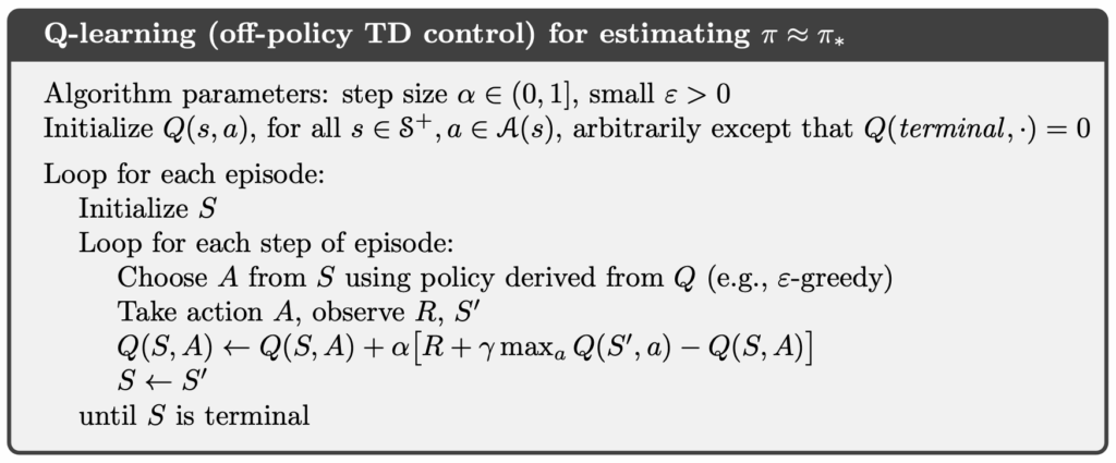
The complete Q-learning algorithm is presented below.

Q-Learning, Off-Policy TD Control (source: Reinforcement Learning: An Introduction, 2nd).

Expected Sarsa (On-Policy/Off-Policy Temporal Difference Control)

Compared with Sarsa, which uses the actually executed next action $Q(S_{t+1}, A_{t+1})$ , and Q-learning, which uses the maximum action-value in the next state $\max_a Q(S_{t+1}, a)$ , Expected Sarsa instead takes the expectation of the action-values in the next state. Its update rule is given by:

$\displaystyle Q(S_t, A_t) \leftarrow Q(S_t, A_t) + \alpha [R_{t+1} + \gamma \mathbb{E}_\pi [Q(S_{t+1}, A_{t+1}) \mid S_{t+1}] - Q(S_t, A_t)] \\\\ \hphantom{Q(S_t, A_t)} \leftarrow Q(S_t, A_t) + \alpha [R_{t+1} + \gamma \sum_a \pi(a \mid S_{t+1}) Q(S_{t+1}, a) - Q(S_t, A_t)]$

By explicitly incorporating the policy $\pi$ into the expectation over actions, Expected Sarsa defines an update target that lies between those of Sarsa and Q-learning. When the policy $\pi$ is $\varepsilon$-greedy and $\varepsilon$ is relatively large, the expectation strongly reflects exploratory behavior. In this case, Expected Sarsa is an on-policy method and exhibits behavior similar to Sarsa, tending to be more conservative.

As $\varepsilon$ is gradually reduced, the $\varepsilon$-greedy policy approaches the greedy policy, and the influence of exploration on the expectation diminishes accordingly. If, at the same time, the behavior policy remains exploratory, a mismatch arises between the policy used to compute the expectation and the policy that actually generates behavior. Expected Sarsa then becomes an off-policy method. Under this setting, its update target gradually approaches that of Q-learning, and it can be viewed as a continuous generalization of Q-learning.

Aside from a modest increase in computational cost, Expected Sarsa often achieves a favorable balance between learning stability and convergence efficiency. For this reason, it is commonly regarded in practice as a TD control method that both encompasses and improves upon Sarsa and Q-learning.

Example of Sarsa

Implementation of Sarsa

In the following code, we implement the Sarsa method faithfully.

In the code, env is a Gymnasium Env object. Gymnasium is the successor to OpenAI Gym and provides a wide range of reinforcement learning environments, allowing us to test RL algorithms in simulated settings.

The environment contains env.observation_space.n states. Accordingly, states are indexed by integers from 0 to env.observation_space.n - 1. The variable Q is a two-dimensional array of floating-point values, where each element corresponds to the estimated action-value of a particular state–action pair. For example, Q[0][0] represents the estimated action-value for taking action 0 in state 0.

import gymnasium as gym
import numpy as np


class Sarsa:
    def __init__(self, env: gym.Env, alpha=0.5, gamma=1.0, epsilon=0.1):
        self.env = env
        self.alpha = alpha
        self.gamma = gamma
        self.epsilon = epsilon

    def _random_argmax(self, q_s: np.ndarray) -> int:
        ties = np.flatnonzero(np.isclose(q_s, q_s.max()))
        return np.random.choice(ties)

    def _epsilon_greedy_action(self, Q: np.ndarray, s: int) -> int:
        if np.random.rand() < self.epsilon:
            return np.random.choice(self.env.action_space.n)
        else:
            ties = np.flatnonzero(np.isclose(Q[s], Q[s].max()))
            return np.random.choice(ties)

    def _create_pi_by_Q(self, Q: np.ndarray) -> np.ndarray:
        pi = np.zeros((self.env.observation_space.n, self.env.action_space.n), dtype=float)
        for s in range(self.env.observation_space.n):
            A_start = self._random_argmax(Q[s])
            pi[s][A_start] = 1.0
        return pi

    def run_control(self, n_episodes=5000) -> tuple[np.ndarray, np.ndarray]:
        Q = np.zeros((self.env.observation_space.n, self.env.action_space.n), dtype=float)

        for i_episode in range(1, n_episodes + 1):
            print(f"\rEpisode: {i_episode}/{n_episodes}", end="", flush=True)

            s, _ = self.env.reset()
            a = self._epsilon_greedy_action(Q, s)

            terminated = False
            truncated = False
            while not (terminated or truncated):
                s_prime, r, terminated, truncated, _ = self.env.step(a)
                a_prime = self._epsilon_greedy_action(Q, s_prime)
                if terminated or truncated:
                    Q[s, a] = Q[s, a] + self.alpha * (r + self.gamma * 0 - Q[s, a])
                else:
                    Q[s, a] = Q[s, a] + self.alpha * (r + self.gamma * Q[s_prime, a_prime] - Q[s, a])
                s = s_prime
                a = a_prime

        pi = self._create_pi_by_Q(Q)
        print()
        return pi, Q

Cliff Walking

Cliff Walking involves moving from a start position to a goal position in a grid world while avoiding falling off a cliff, as illustrated below.

In the Cliff Walking problem, each state corresponds to the player’s current position. There are a total of 36 states, consisting of the top three rows plus the bottom-left cell, giving $3 \times 12 + 1 = 36$ states. The current position is computed using the following formula:

$\text{position} = \text{current-row} \times \text{num-col} + \text{current-col}$

There are four available actions:

0: Move up
1: Move right
2: Move down
3: Move left

Each step yields a reward of −1. However, if the agent steps into the cliff, it receives a reward of −100.

import time

import gymnasium as gym
import numpy as np

from expected_sarsa import ExpectedSarsa
from q_learning import QLearning
from sarsa import Sarsa

GYM_ID = "CliffWalking-v1"


def play_game(policy, episodes=1):
    visual_env = gym.make(GYM_ID, render_mode="human")

    for episode in range(episodes):
        state, _ = visual_env.reset()
        terminated = False
        truncated = False
        total_reward = 0
        step_count = 0

        for i in range(10):
            print(f"Sleep {i}")
            time.sleep(1)

        print(f"Episode {episode + 1} starts")
        while not terminated and not truncated:
            action = np.argmax(policy[state])
            state, reward, terminated, truncated, _ = visual_env.step(action)
            total_reward += reward
            step_count += 1
            time.sleep(0.3)

        print(f"Episode {episode + 1} is finished: Total reward is {total_reward}, steps = {step_count}")
        time.sleep(1)

    visual_env.close()


if __name__ == "__main__":
    env = gym.make(GYM_ID)

    print(f"Gym environment: {GYM_ID}")

    print("Start Sarsa")
    sarsa = Sarsa(env)
    sarsa_policy, sarsa_Q = sarsa.run_control()
    play_game(sarsa_policy)
    print("\n")

    env.close()

Below are the results produced by the above code. We can observe that the agent does not choose the shortest path that runs close to the cliff. Instead, it tends to follow a route that stays farther away from the cliff and involves lower risk. This behavior arises because Sarsa updates its action-value estimates using the next action actually sampled by the same $\varepsilon$-greedy policy. As a result, the risk introduced by exploratory actions is directly reflected in the value estimates. Consequently, in high-risk environments such as Cliff Walking, Sarsa naturally learns more conservative yet stable policies.

Taxi

The Taxi problem takes place in a grid world where the agent must navigate to the passenger’s location, pick up the passenger, and then deliver them to one of four designated destinations, as illustrated below.

In the Taxi problem, there are 500 discrete states. Each state is encoded by the following formula:

$r: \text{the row the taxi is currently at} \\\\ c: \text{the colunm the taxi is currently at} \\\\ p: \text{the location the passenger is at} \\\\ d: \text{the destination to drop off the passenger} \\\\ state = ((r \times 5 + c) \times 5 + p) * 4 + d$

Passenger locations are defined as:

0: Red
1: Green
2: Yellow
3: Blue
4: In taxi

Destinations are defined as:

0: Red
1: Green
2: Yellow
3: Blue

There are six available actions:

0: Move south (down)
1: Move north (up)
2: Move east (right)
3: Move west (left)
4: Pick up passenger
5: Drop off passenger

Each step yields a reward of −1 unless another reward is triggered. Successfully delivering the passenger to the destination yields a reward of +20. Executing an illegal pickup or drop-off action results in a reward of −10.

import time

import gymnasium as gym
import numpy as np

from expected_sarsa import ExpectedSarsa
from q_learning import QLearning
from sarsa import Sarsa

GYM_ID = "Taxi-v3"


def play_game(policy, episodes=1):
    visual_env = gym.make(GYM_ID, render_mode="human")

    for episode in range(episodes):
        state, _ = visual_env.reset()
        terminated = False
        truncated = False
        total_reward = 0
        step_count = 0

        for i in range(10):
            print(f"Sleep {i}")
            time.sleep(1)

        print(f"Episode {episode + 1} starts")
        while not terminated and not truncated:
            action = np.argmax(policy[state])
            state, reward, terminated, truncated, _ = visual_env.step(action)
            total_reward += reward
            step_count += 1
            time.sleep(0.3)

        print(f"Episode {episode + 1} is finished: Total reward is {total_reward}, steps = {step_count}")
        time.sleep(1)

    visual_env.close()


if __name__ == "__main__":
    env = gym.make(GYM_ID)

    print(f"Gym environment: {GYM_ID}")

    print("Start Sarsa")
    sarsa = Sarsa(env)
    sarsa_policy, sarsa_Q = sarsa.run_control()
    play_game(sarsa_policy)
    print("\n")

    env.close()

Below are the execution results of the above program.

Example of Q-Learning

Implementation of Q-Learning

In the following code, we faithfully implement the Q-Learning method.

import gymnasium as gym
import numpy as np


class QLearning:
    def __init__(self, env: gym.Env, alpha=0.5, gamma=1.0, epsilon=0.1):
        self.env = env
        self.alpha = alpha
        self.gamma = gamma
        self.epsilon = epsilon

    def _random_argmax(self, q_s: np.ndarray) -> int:
        ties = np.flatnonzero(np.isclose(q_s, q_s.max()))
        return np.random.choice(ties)

    def _epsilon_greedy_action(self, Q: np.ndarray, s: int) -> int:
        if np.random.rand() < self.epsilon:
            return np.random.choice(self.env.action_space.n)
        else:
            ties = np.flatnonzero(np.isclose(Q[s], Q[s].max()))
            return np.random.choice(ties)

    def _create_pi_by_Q(self, Q: np.ndarray) -> np.ndarray:
        pi = np.zeros((self.env.observation_space.n, self.env.action_space.n), dtype=float)
        for s in range(self.env.observation_space.n):
            A_start = self._random_argmax(Q[s])
            pi[s][A_start] = 1.0
        return pi

    def run_control(self, n_episode=5000) -> tuple[np.ndarray, np.ndarray]:
        Q = np.zeros((self.env.observation_space.n, self.env.action_space.n), dtype=float)

        for i_episode in range(1, n_episode + 1):
            print(f"\rEpisode: {i_episode}/{n_episode}", end="", flush=True)

            s, _ = self.env.reset()

            terminated = False
            truncated = False
            while not (terminated or truncated):
                a = self._epsilon_greedy_action(Q, s)
                s_prime, r, terminated, truncated, _ = self.env.step(a)
                if terminated or truncated:
                    Q[s, a] = Q[s, a] + self.alpha * (r + self.gamma * 0 - Q[s, a])
                else:
                    Q[s, a] = Q[s, a] + self.alpha * (r + self.gamma * np.max(Q[s_prime]) - Q[s, a])
                s = s_prime

        pi = self._create_pi_by_Q(Q)
        print()
        return pi, Q

Cliff Walking

In the following, we use Q-Learning to solve the Cliff Walking problem.

import time

import gymnasium as gym
import numpy as np

from expected_sarsa import ExpectedSarsa
from q_learning import QLearning
from sarsa import Sarsa

GYM_ID = "CliffWalking-v1"


def play_game(policy, episodes=1):
    visual_env = gym.make(GYM_ID, render_mode="human")

    for episode in range(episodes):
        state, _ = visual_env.reset()
        terminated = False
        truncated = False
        total_reward = 0
        step_count = 0

        for i in range(10):
            print(f"Sleep {i}")
            time.sleep(1)

        print(f"Episode {episode + 1} starts")
        while not terminated and not truncated:
            action = np.argmax(policy[state])
            state, reward, terminated, truncated, _ = visual_env.step(action)
            total_reward += reward
            step_count += 1
            time.sleep(0.3)

        print(f"Episode {episode + 1} is finished: Total reward is {total_reward}, steps = {step_count}")
        time.sleep(1)

    visual_env.close()


if __name__ == "__main__":
    env = gym.make(GYM_ID)

    print(f"Gym environment: {GYM_ID}")

    print("Start Q-learning")
    q_learning = QLearning(env)
    ql_policy, ql_Q = q_learning.run_control()
    play_game(ql_policy)
    print("\n")

    env.close()

Below are the results produced by the above code. We can observe that the agent learns the shortest path that runs close to the cliff. This is because Q-learning uses $\max_a Q(S_{t+1}, a)$ as the TD target when updating action-value estimates, without accounting for the risk introduced by actual exploratory behavior. As a result, Q-learning directly approximates the optimal action-value function $q_*$ . While this leads to higher efficiency during evaluation, it also makes the agent more prone to falling into the cliff due to exploration during training.

Taxi

In the following, we use Q-Learning to solve the Taxi problem.

import time

import gymnasium as gym
import numpy as np

from expected_sarsa import ExpectedSarsa
from q_learning import QLearning
from sarsa import Sarsa

GYM_ID = "Taxi-v3"


def play_game(policy, episodes=1):
    visual_env = gym.make(GYM_ID, render_mode="human")

    for episode in range(episodes):
        state, _ = visual_env.reset()
        terminated = False
        truncated = False
        total_reward = 0
        step_count = 0

        for i in range(10):
            print(f"Sleep {i}")
            time.sleep(1)

        print(f"Episode {episode + 1} starts")
        while not terminated and not truncated:
            action = np.argmax(policy[state])
            state, reward, terminated, truncated, _ = visual_env.step(action)
            total_reward += reward
            step_count += 1
            time.sleep(0.3)

        print(f"Episode {episode + 1} is finished: Total reward is {total_reward}, steps = {step_count}")
        time.sleep(1)

    visual_env.close()


if __name__ == "__main__":
    env = gym.make(GYM_ID)

    print(f"Gym environment: {GYM_ID}")

    print("Start Q-learning")
    q_learning = QLearning(env)
    ql_policy, ql_Q = q_learning.run_control()
    play_game(ql_policy)
    print("\n")

    env.close()

Below are the execution results of the above program.

Example of Expected Sarsa

Implementation of Expected Sarsa

In the following code, we faithfully implement the Expected Sarsa method.

import gymnasium as gym
import numpy as np


class ExpectedSarsa:
    def __init__(self, env: gym.Env, alpha=0.5, gamma=1.0, epsilon=0.1):
        self.env = env
        self.alpha = alpha
        self.gamma = gamma
        self.epsilon = epsilon

    def _random_argmax(self, q_s: np.ndarray) -> int:
        ties = np.flatnonzero(np.isclose(q_s, q_s.max()))
        return np.random.choice(ties)

    def _epsilon_greedy_action(self, Q: np.ndarray, s: int) -> int:
        if np.random.rand() < self.epsilon:
            return np.random.choice(self.env.action_space.n)
        else:
            ties = np.flatnonzero(np.isclose(Q[s], Q[s].max()))
            return np.random.choice(ties)

    def _epsilon_greedy_probabilities(self, q_s: np.ndarray):
        probs = np.ones(self.env.action_space.n, dtype=float) * (self.epsilon / self.env.action_space.n)
        max_q = np.max(q_s)
        greedy_actions = np.flatnonzero(np.isclose(q_s, max_q))
        probs[greedy_actions] += (1 - self.epsilon) / len(greedy_actions)
        return probs

    def _create_pi_by_Q(self, Q: np.ndarray) -> np.ndarray:
        pi = np.zeros((self.env.observation_space.n, self.env.action_space.n), dtype=float)
        for s in range(self.env.observation_space.n):
            A_start = self._random_argmax(Q[s])
            pi[s][A_start] = 1.0
        return pi

    def run_control(self, n_episodes=5000):
        Q = np.zeros((self.env.observation_space.n, self.env.action_space.n), dtype=float)

        for i_episode in range(1, n_episodes + 1):
            print(f"\rEpisode: {i_episode}/{n_episodes}", end="", flush=True)

            s, _ = self.env.reset()

            terminated = False
            truncated = False
            while not (terminated or truncated):
                a = self._epsilon_greedy_action(Q, s)
                s_prime, r, terminated, truncated, _ = self.env.step(a)
                if terminated or truncated:
                    Q[s, a] = Q[s, a] + self.alpha * (r + self.gamma * 0 - Q[s, a])
                else:
                    expectation = np.dot(self._epsilon_greedy_probabilities(Q[s_prime]), Q[s_prime])
                    Q[s, a] = Q[s, a] + self.alpha * (r + self.gamma * expectation - Q[s, a])
                s = s_prime

        pi = self._create_pi_by_Q(Q)
        print()
        return pi, Q

Cliff Walking

Next, we use Expected Sarsa to solve the Cliff Walking problem. We ran two experiments, using $\varepsilon = 0.1$ and $\varepsilon = 0.001$ , respectively.

import time

import gymnasium as gym
import numpy as np

from expected_sarsa import ExpectedSarsa
from q_learning import QLearning
from sarsa import Sarsa

GYM_ID = "CliffWalking-v1"


def play_game(policy, episodes=1):
    visual_env = gym.make(GYM_ID, render_mode="human")

    for episode in range(episodes):
        state, _ = visual_env.reset()
        terminated = False
        truncated = False
        total_reward = 0
        step_count = 0

        for i in range(10):
            print(f"Sleep {i}")
            time.sleep(1)

        print(f"Episode {episode + 1} starts")
        while not terminated and not truncated:
            action = np.argmax(policy[state])
            state, reward, terminated, truncated, _ = visual_env.step(action)
            total_reward += reward
            step_count += 1
            time.sleep(0.3)

        print(f"Episode {episode + 1} is finished: Total reward is {total_reward}, steps = {step_count}")
        time.sleep(1)

    visual_env.close()


if __name__ == "__main__":
    env = gym.make(GYM_ID)

    print(f"Gym environment: {GYM_ID}")

    print("Start Expected Sarsa with epsilon = 0.1")
    esarsa_01 = ExpectedSarsa(env, epsilon=0.1)
    esarsa_01_policy, esarsa_01_Q = esarsa_01.run_control()
    play_game(esarsa_01_policy)
    print("\n")

    print("Start Expected Sarsa with epsilon = 0.001")
    esarsa_0001 = ExpectedSarsa(env, epsilon=0.001)
    esarsa_0001_policy, esarsa_0001_Q = esarsa_0001.run_control()
    play_game(esarsa_0001_policy)
    print("\n")

    env.close()

Below are the results produced by the above code. Unlike Sarsa and Q-learning, Expected Sarsa updates action-value estimates by taking the expectation over the values of all possible actions in the next state, which effectively incorporates the risk of exploration in an averaged manner.

When $\varepsilon$ is relatively large (e.g., 0.1), the agent recognizes that it may slip due to exploratory actions with a non-trivial probability (10%). As a result, it tends to favor safer routes that stay farther away from the cliff. When $\varepsilon$ is extremely small (e.g., 0.001), the agent effectively assumes that slipping is almost impossible (0.01%), so the exploration risk becomes negligible. In expectation, moving along the cliff edge remains the most cost-effective strategy, and the learned behavior begins to hug the cliff more closely.

From this perspective, Expected Sarsa transitions smoothly between risk awareness and efficiency prioritization as $\varepsilon$ changes, forming a natural compromise between Sarsa and Q-learning.

Cliff Walking by Expected Sarsa with epsilon 0.1.

Cliff Walking by Expected Sarsa with epsilon 0.001.

Taxi

Next, we use Expected Sarsa to solve the Taxi problem. We ran two experiments, using $\varepsilon = 0.1$ and $\varepsilon = 0.001$ , respectively.

import time

import gymnasium as gym
import numpy as np

from expected_sarsa import ExpectedSarsa
from q_learning import QLearning
from sarsa import Sarsa

GYM_ID = "Taxi-v3"


def play_game(policy, episodes=1):
    visual_env = gym.make(GYM_ID, render_mode="human")

    for episode in range(episodes):
        state, _ = visual_env.reset()
        terminated = False
        truncated = False
        total_reward = 0
        step_count = 0

        for i in range(10):
            print(f"Sleep {i}")
            time.sleep(1)

        print(f"Episode {episode + 1} starts")
        while not terminated and not truncated:
            action = np.argmax(policy[state])
            state, reward, terminated, truncated, _ = visual_env.step(action)
            total_reward += reward
            step_count += 1
            time.sleep(0.3)

        print(f"Episode {episode + 1} is finished: Total reward is {total_reward}, steps = {step_count}")
        time.sleep(1)

    visual_env.close()


if __name__ == "__main__":
    env = gym.make(GYM_ID)

    print(f"Gym environment: {GYM_ID}")

    print("Start Expected Sarsa with epsilon = 0.1")
    esarsa_01 = ExpectedSarsa(env, epsilon=0.1)
    esarsa_01_policy, esarsa_01_Q = esarsa_01.run_control()
    play_game(esarsa_01_policy)
    print("\n")

    print("Start Expected Sarsa with epsilon = 0.001")
    esarsa_0001 = ExpectedSarsa(env, epsilon=0.001)
    esarsa_0001_policy, esarsa_0001_Q = esarsa_0001.run_control()
    play_game(esarsa_0001_policy)
    print("\n")

    env.close()

Below are the execution results of the above program.

Taxi by Expected Sarsa with epsilon 0.1.

Taxi by Expected Sarsa with epsilon 0.001.

Conclusion

This chapter introduced TD prediction and three TD control methods. Although they differ in form, they are all fundamentally built upon the same incremental update framework. The differences among Sarsa, Q-learning, and Expected Sarsa do not lie in the learning procedure itself, but in how the update target is defined and in the trade-off between on-policy and off-policy learning. From this unified perspective, TD control is no longer a collection of isolated algorithms, but rather a continuous family of learning methods that can be directly compared and understood in relation to one another.

References

Adam White and Martha White. Reinforcement Learning Specialization. University of Alberta and Coursera.
Richard S. Sutton and Andrew G. Barto. 2020. Reinforcement Learning: An Introduction, 2^nd. The MIT Press.

Temporal-Difference Learning, TD

Share

Table of Contents

Incremental Implementation

Temporal Difference, TD

Temporal Difference Prediction

One-Step Temporal Difference, TD(0)

Temporal Difference Control

Sarsa (On-Policy Temporal Difference Control)

Q-Learning (Off-Policy Temporal Difference Control)

Expected Sarsa (On-Policy/Off-Policy Temporal Difference Control)

Example of Sarsa

Implementation of Sarsa

Cliff Walking

Taxi

Example of Q-Learning

Implementation of Q-Learning

Cliff Walking

Taxi

Example of Expected Sarsa

Implementation of Expected Sarsa

Cliff Walking

Taxi

Conclusion

References

Related Tags

Leave a Reply Cancel reply

You May Also Like