Monte Carlo Methods, MC

In Dynamic Programming (DP), having a complete environment model is a prerequisite for exact computation. However, this assumption rarely holds in most real-world problems. Monte Carlo Methods (MC) methods choose to forgo reliance on an explicit model and instead learn directly from complete experiences generated through interaction with the environment. By sampling and averaging episode returns, MC provides a practical pathway for estimating value functions grounded in actual experience.

The complete code for this chapter can be found in .

Monte Carlo, MC

Dynamic Programming (DP) requires a complete environment model, an assumption that is almost impossible to satisfy in real-world environments. Monte Carlo Methods (MC) methods, in contrast, form a class of approaches that do not rely on an environment model. Instead, they estimate value functions directly from return samples obtained from complete episodes generated through actual interaction with the environment, and therefore do not require a model. In other words, MC is a model-free method.

To define returns unambiguously, we focus on MC methods formulated for episodic tasks. That is, experience is assumed to be divided into multiple episodes, and all episodes are guaranteed to terminate. MC methods sample these episodes and estimate the value function by averaging the observed returns. Consequently, MC is a non-bootstrapping method.

On-Policy Monte Carlo

On-policy refers to the setting in MC methods where the policy used to generate data is the same policy that is being evaluated and improved. In other words, the behavior policy $b$ and the target policy $\pi$ are identical.

On-Policy Monte Carlo Prediction

The value of a state is the expected return obtainable starting from that state, that is, the expectation of the future discounted cumulative reward.

$\displaystyle v_\pi(s) \doteq \mathbb{E}_\pi \left[ G_t \mid S_t=s \right] \\\\ G_t = \sum_{k=0}^{T-t-1} \gamma^k R_{t+k+1}$

Since a value is, by definition, an expected return, it can be estimated by sampling the returns actually observed and averaging them. As the number of observed returns increases, this average should converge to the corresponding expectation. This idea forms the foundation of all MC methods.

$\displaystyle v_\pi(s) \approx \frac{1}{N(s)} \sum_{i=1}^{N(s)} G_t^{(i)}$

We will introduce two on-policy MC prediction methods. Their main difference lies in how samples are collected, but both converge to $v_\pi$ .

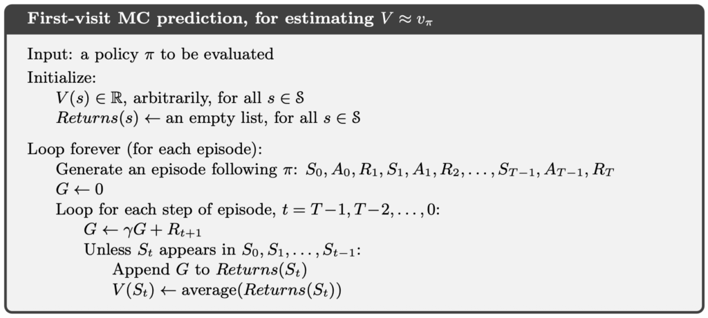
First-Visit Monte Carlo Prediction

First-Visit MC Prediction updates a state only on its first occurrence within each episode. At the beginning of each iteration, the agent interacts with the environment to generate an episode. It then proceeds to sample returns from that episode and uses them to update the value estimates.

Every-Visit Monte Carlo Prediction

Every-Visit MC Prediction updates a state whenever it is encountered, regardless of whether it is the first occurrence within the episode. The Every-Visit MC Prediction algorithm is almost identical to First-Visit MC Prediction; the key difference is that, during sampling, it does not perform the check “Unless $S_t$ appears in $S_0, S_1, \cdots, S_{t-1}$ .”

On-Policy Monte Carlo Control

DP can use $v(s)$ for control because it has access to a model $p(s^\prime, r \mid s, a)$ , which allows the expectation over actions to be computed explicitly.

MC methods, however, are model-free and therefore lack the transition dynamics $p(s^\prime, r \mid s, a)$ . As a result, they cannot compute expectations over actions. Instead, the experience generated through interaction with the environment contains data from actions that were actually taken, $(s, a)$ , which can be used to compute returns.

Consequently, under MC methods, the control problem must shift to learning the action-value function $q_\pi(s, a)$ , rather than operating directly on $v(s)$ . For each state, actions are then selected deterministically in a greedy manner by choosing the action with the highest action value. Policy improvement can be achieved by constructing each $\pi_{k+1}$ as the greedy policy with respect to $q_{\pi_k}$ . In this setting, the policy improvement theorem applies to $\pi_k$ and $\pi_{k+1}$ .

$\pi_{k+1}(s) \doteq \text{argmax}_a q_{\pi_k}(s, a)$

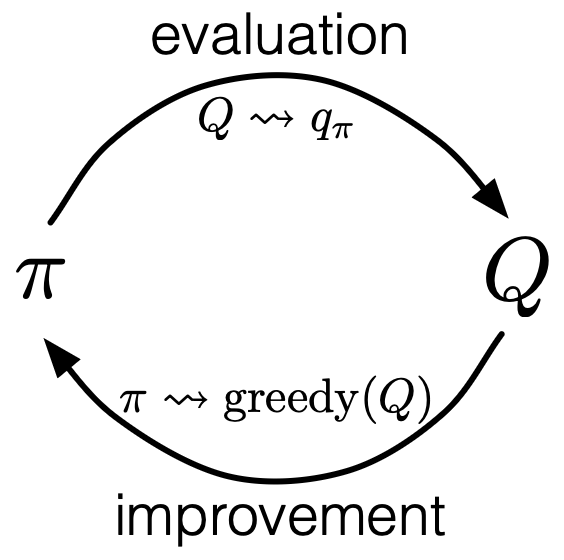
From the perspective of Generalized Policy Iteration (GPI), MC control consists of repeatedly estimating $q_\pi$ using MC methods and applying policy improvement to push the policy toward better solutions.

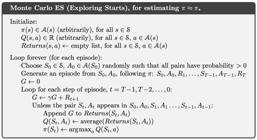
Monte Carlo Control (source: Reinforcement Learning: An Introduction, 2nd).

Monte Carlo with Exploring Starts, MCES

MC control aims to learn $q_*$ . However, MC methods can only learn from state–action pairs $(s, a)$ that are actually visited. Any $(s, a)$ that is never encountered will therefore never be learned.

$\displaystyle q_*(s, a) = \max_\pi q_\pi(s, a)$

To address this issue, Monte Carlo with Exploring Starts (MCES) ensures that every state–action pair $(s, a)$ has a nonzero probability of being selected as the starting point of an episode, thereby guaranteeing that all $(s, a)$ pairs are visited infinitely often.

Before generating an episode, MCES first randomly selects a state–action pair $(s, a)$ as the starting point, and then generates the episode from that initial condition.

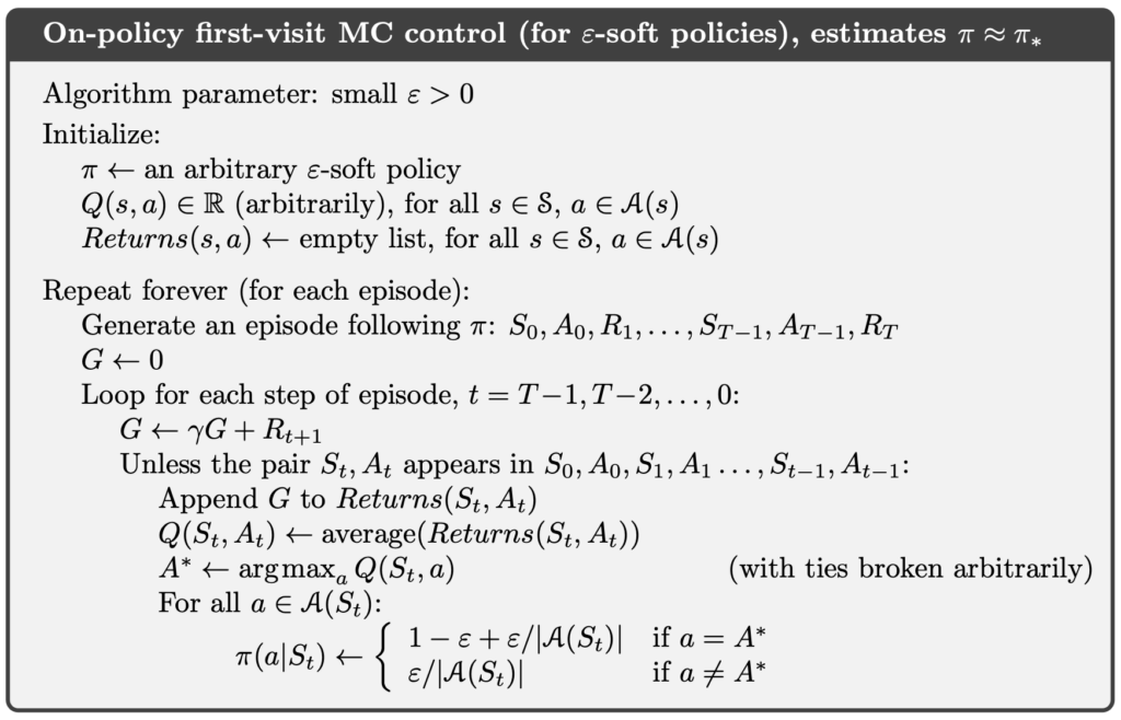
Monte Carlo with Exploring Starts, MCES (source: Reinforcement Learning: An Introduction, 2nd).

On-Policy First-Visit Monte Carlo (ε-soft policies)

The exploring starts assumption in MCES is impractical. In practice, it is almost impossible to arbitrarily specify the starting point of an episode. Therefore, we need an approach that does not rely on the exploring starts assumption while still guaranteeing sufficient exploration.

An $\varepsilon$ -soft policy is defined such that, for any state $s$ , all possible actions $a$ have a nonzero probability of being selected, and thus are never permanently eliminated through policy improvement.

$\pi(a \mid s) \ge \frac{\varepsilon}{|\mathcal{A}(s)|}$

In the final step of the algorithm, MCES updates $\pi(S_t)$ using a deterministic greedy policy. As a result, only the action $a$ with the highest action value is assigned probability 1, while all other actions receive probability 0. In contrast, when updating $\pi(S_t)$ using an $\varepsilon$ -soft policy, the action $a$ with the highest action value is assigned probability $1 - \varepsilon + \frac{\varepsilon}{|\mathcal{A}(S_t)|}$ , and all other actions are assigned probability $\frac{\varepsilon}{|\mathcal{A}(S_t)|}$ .

On-Policy First-Visit Monte Carlo Control (source: Reinforcement Learning: An Introduction, 2nd).

Off-Policy Monte Carlo

The on-policy methods described above require that data generation be consistent with the policy being learned. However, in practice, this assumption is often difficult to satisfy, which motivates the introduction of an off-policy learning framework.

Importance Sampling

In off-policy learning, we encounter a structural issue, that is data are generated by a behavior policy $b$ , while the objective is to evaluate or learn a target policy $\pi$ .

$\text{Sample}: x \sim b \\ \text{Estimate}: \mathbb{E}_\pi \left[ X \right]$

However, expectations cannot be transferred directly across different distributions. Therefore, importance sampling is required to correct the bias caused by this distribution mismatch.

Importance sampling is a general technique for estimating the expectation under a target distribution when samples are drawn from a different distribution. In off-policy learning, importance sampling is applied by weighting returns according to the relative probability of the same trajectory occurring under the target policy and the behavior policy. This relative probability ratio is called the importance-sampling ratio $\rho$ .

$\rho(x) = \frac{\pi(x)}{b(x)}$

The following derivation shows how the expectation under the target policy $\pi$ can be expressed in terms of the expectation under the behavior policy $b$ .

$\displaystyle \mathbb{E}_\pi \left[ X \right] \doteq \sum_{x \in X} x\pi(x) \\\\ \hphantom{\mathbb{E}_\pi \left[ X \right]} = \sum_{x \in X} x\pi(x) \frac{b(x)}{b(x)} \\\\ \hphantom{\mathbb{E}_\pi \left[ X \right]} = \sum_{x \in X} x \frac{\pi(x)}{b(x)} b(x) \\\\ \hphantom{\mathbb{E}_\pi \left[ X \right]} = \sum_{x \in X} x \rho(x) b(x) \\\\ \hphantom{\mathbb{E}_\pi \left[ X \right]} = \mathbb{E}_b \left[ X \rho(X) \right]$

Next, we approximate $\mathbb{E}_b \left[ X \rho(X) \right]$ :

$\displaystyle \mathbb{E} \left[ X \right] \approx \frac{1}{n} \sum_{i=1}^n x_i \\\\ \mathbb{E}_b \left[ X \rho(X) \right] \doteq \sum_{x \in X} x\rho(x)b(x) \\\\ \hphantom{\mathbb{E}_b \left[ X \rho(X) \right]} \approx \frac{1}{n} \sum_{i=1}^n x_i \rho_(x_i)$

Finally, we obtain an approximation of $\mathbb{E}_\pi \left[ X \right]$ :

$\displaystyle \mathbb{E}_\pi \left[ X \right] \approx \frac{1}{n} \sum_{i=1}^n x_i \rho(x_i), \quad x_i \sim b$

It is important to note that although importance sampling can correct for distribution mismatch, its variance can be very large, especially when trajectories are long or when the behavior and target policies differ significantly.

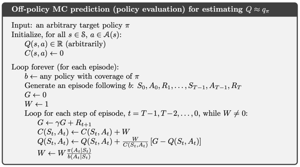
Off-Policy Monte Carlo Prediction

Given a starting state $S_t$ , the subsequent trajectory is $A_t, S_{t+1}, A_{t+1}, \cdots, S_T$ . Under an arbitrary policy $\pi$ , the probability of this trajectory can be written as:

$\displaystyle \text{Pr}\{A_t, S_{t+1}, A_{t+1}, \cdots, S_T \mid S_t, A_{t:T-1} \sim \pi\} \\\\ = \pi(A_t \mid S_t) p(S_{t+1} \mid S_t, A_t) \pi(A_{t+1} \mid S_{t+1}) \cdots p(S_T \mid S_{T-1}, A_{T-1}) \\\\ = \prod_{k=t}^{T-1} \pi(A_k \mid S_k) p(S_{k+1} \mid S_k, A_k)$

Accordingly, the importance-sampling ratio from time step $t$ to the end of the episode, $\rho_{t:T-1}$ , is defined as:

$\displaystyle \rho_{t:T-1} \doteq \frac{\displaystyle \prod_{k=t}^{T-1} \pi(A_k \mid S_k) p(S_{k+1} \mid S_k, A_k)}{\displaystyle \prod_{k=t}^{T-1} b(A_k \mid S_k) p(S_{k+1} \mid S_k, A_k)} = \prod_{k=t}^{T-1} \frac{\pi(A_k \mid S_k)}{b(A_k \mid S_k)}$

Under the behavior policy $b$ , the expectation over all returns $G_t$ corresponds to $v_b(s)$ :

$\mathbb{E}_b \left[ G_t \mid S_t=s \right]=v_b(s)$

However, returns $G_t$ generated by the behavior policy $b$ cannot be used directly to estimate $v_\pi(s)$ . By applying the importance-sampling ratio $\rho_{t:T-1}$ , $G_t$ can be transformed into an unbiased estimate under the target policy $\pi$ :

$\mathbb{E} \left[\rho_{t:T-1} G_t \mid S_t=s \right] = v_\pi(s)$

The importance-sampling ratio $\rho_{t:T-1}$ can be computed incrementally:

$\displaystyle \rho_{t:T-1} = \prod_{k=t}^{T-1} \frac{\pi(A_k \mid S_k)}{b(A_k \mid S_k)} \\\\ \hphantom{\rho_{t:T-1}} = \rho_t \rho_{t+1} \rho_{t+1} \cdots \rho_{T-2}\rho_{T-1} \\\\ W_1 \leftarrow \rho_{T-1} \\\\ W_2 \leftarrow \rho_{T-1} \rho_{T-2} \\\\ W_3 \leftarrow \rho_{T-1} \rho_{T-2} \rho_{T-3} \\\\ W_{t+1} \leftarrow W_t \rho_t$

Here, $W_t$ can be viewed as the weight associated with the return $G_t$ . Suppose we observe a sequence of returns $G_1, G_2, \cdots, G_{n-1}$ starting from the same state, each with a corresponding weight $W_i$ . The state-value estimate can then be expressed as a weighted average:

$V_n \doteq \frac{\displaystyle \sum_{k=1}^{n-1} W_k G_k}{\displaystyle \sum_{k=1}^{n-1} W_k}, \quad n \ge 2$

When a new return $G_n$ is obtained, $V_n$ is updated. To do so, in addition to tracking $V_n$ , we also maintain the cumulative sum of weights $C_n$ :

$C_{n+1} \doteq C_n + W_{n+1}$

The corresponding incremental update rule is:

$V_{n+1} \doteq V_n + \frac{W_n}{C_n} \left[ G_n - V_n \right], \quad n \ge 1$

The above derivation and update rules constitute the off-policy MC prediction algorithm.

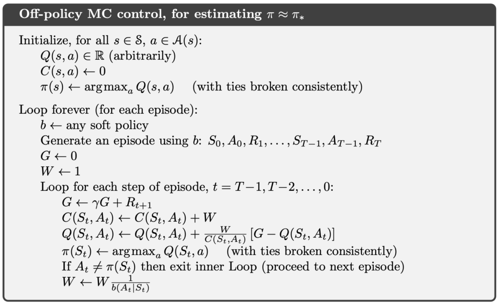
Off-Policy Monte Carlo Prediction (source: Reinforcement Learning: An Introduction, 2nd).

Off-Policy Monte Carlo Control

The objective of off-policy MC control is to learn

$q_*(s, a) = \max_\pi q_\pi(s, a)$

In this setting, the behavior policy $b$ must be an $\varepsilon$ -soft policy, while the target policy $\pi$ is the greedy policy with respect to $Q$ , where $Q$ is an estimate of $q_\pi$ .

Off-Policy Monte Carlo Control (source: Reinforcement Learning: An Introduction, 2nd).

Example of On-Policy Monte Carlo

Implementation of On-Policy First-Visit Monte Carlo Control (ε-soft policies)

In the following code, we faithfully implement the on-policy first-visit MC control method with $\varepsilon$ -soft policies.

In the code, env is a Gymnasium Env object. Gymnasium is the successor to OpenAI Gym and provides a wide collection of reinforcement learning environments, allowing us to test RL algorithms in simulated settings.

An environment contains env.observation_space.n states. Accordingly, states are indexed by integers from 0 to env.observation_space.n - 1. The variable Q is a two-dimensional array of floating-point numbers, where each element represents an estimate of the action value for a specific state–action pair. For example, Q[0][0] denotes the estimated action value of action 0 in state 0.

import gymnasium as gym
import numpy as np


class OnPolicyMonteCarlo:
    def __init__(self, env: gym.Env, epsilon=0.1, gamma=1.0):
        self.env = env
        self.epsilon = epsilon
        self.gamma = gamma

    def _random_argmax(self, q_s: np.ndarray) -> int:
        ties = np.flatnonzero(np.isclose(q_s, q_s.max()))
        return np.random.choice(ties)

    def _update_policy_for_state(self, pi: np.ndarray, Q: np.ndarray, s: int):
        A = np.ones(self.env.action_space.n, dtype=float) * self.epsilon / self.env.action_space.n
        A_start = self._random_argmax(Q[s])
        A[A_start] += 1.0 - self.epsilon
        pi[s] = A

    def _update_policy_by_epsilon_greedy(self, pi: np.ndarray, Q: np.ndarray):
        for s in range(self.env.observation_space.n):
            A = np.ones(self.env.action_space.n, dtype=float) * self.epsilon / self.env.action_space.n
            A_star = np.argmax(Q[s])
            A[A_star] += 1.0 - self.epsilon
            pi[s] = A

    def _generate_episode(self, pi: np.ndarray) -> list[tuple[int, int, float]]:
        episode = []
        s, _ = self.env.reset()
        while True:
            a = np.random.choice(np.arange(self.env.action_space.n), p=pi[s])
            s_prime, r, terminated, truncated, _ = self.env.step(a)
            episode.append((s, a, r))

            if terminated or truncated:
                break
            s = s_prime
        return episode

    def run_control(self, n_episodes=5000) -> tuple[np.ndarray, np.ndarray]:
        Q = np.zeros((self.env.observation_space.n, self.env.action_space.n), dtype=float)
        Returns_sum = np.zeros((self.env.observation_space.n, self.env.action_space.n), dtype=float)
        Returns_count = np.zeros((self.env.observation_space.n, self.env.action_space.n), dtype=int)

        pi = np.zeros((self.env.observation_space.n, self.env.action_space.n), dtype=float)
        self._update_policy_by_epsilon_greedy(pi, Q)

        for i_episode in range(1, n_episodes + 1):
            print(f"\rEpisode: {i_episode}/{n_episodes}, generating a episode ...", end="", flush=True)

            episode = self._generate_episode(pi)
            print(f"\rEpisode: {i_episode}/{n_episodes}, episode length is {len(episode)})", end="", flush=True)

            sa_first_visit = {}
            for t, (s, a, _) in enumerate(episode):
                if (s, a) not in sa_first_visit:
                    sa_first_visit[(s, a)] = t

            G = 0.0
            for t in range(len(episode) - 1, -1, -1):
                s, a, r = episode[t]
                G = self.gamma * G + r

                if t == sa_first_visit[(s, a)]:
                    Returns_sum[s, a] += G
                    Returns_count[s, a] += 1
                    Q[s, a] = Returns_sum[s, a] / Returns_count[s, a]
                    self._update_policy_for_state(pi, Q, s)

        print()
        return pi, Q

Cliff Walking

Cliff Walking involves moving from a start position to a goal position in a grid world while avoiding falling off a cliff, as illustrated below.

In the Cliff Walking problem, each state corresponds to the player’s current position. There are a total of 36 states, consisting of the top three rows plus the bottom-left cell, giving $3 \times 12 + 1 = 36$ states. The current position is computed using the following formula:

$\text{position} = \text{current-row} \times \text{num-col} + \text{current-col}$

There are four available actions:

0: Move up
1: Move right
2: Move down
3: Move left

Each step yields a reward of −1. However, if the agent steps into the cliff, it receives a reward of −100.

import numpy as np

from off_policy_mc import OffPolicyMonteCarlo
from on_policy_mc import OnPolicyMonteCarlo

GYM_ID = "CliffWalking-v1"


def play_game(policy, episodes=1):
    visual_env = gym.make(GYM_ID, render_mode="human")

    for episode in range(episodes):
        state, _ = visual_env.reset()
        terminated = False
        truncated = False
        total_reward = 0
        step_count = 0

        print(f"Episode {episode + 1} starts")
        while not terminated and not truncated:
            action = np.argmax(policy[state])
            state, reward, terminated, truncated, _ = visual_env.step(action)
            total_reward += reward
            step_count += 1
            time.sleep(0.3)

        print(f"Episode {episode + 1} is finished: Total reward is {total_reward}, steps = {step_count}")
        time.sleep(1)

    visual_env.close()


if __name__ == "__main__":
    env = gym.make(GYM_ID)

    print(f"Gym environment: {GYM_ID}")

    print("Start On-Policy First-Visit Monte Carlo (for epsilon-soft policies)")
    on_policy_mc = OnPolicyMonteCarlo(env)
    on_policy_pi, on_policy_Q = on_policy_mc.run_control(n_episodes=5000)
    play_game(on_policy_pi)

Below are the execution results of the above program. We can observe that the learned policy typically deliberately avoids the edge of the cliff, choosing a more conservative path with lower risk. Even in the later stages of training, when the value function has largely stabilized, the agent does not tend to move tightly along the cliff.

This behavior is not due to an implementation issue, but rather an inherent characteristic of on-policy MC control. Because the behavior policy is $\varepsilon$-soft, the agent always has a nonzero probability of taking non-greedy actions during execution. When operating near the cliff, such random deviations can immediately lead to falling into the cliff and incurring a large negative reward. As a result, the value estimation naturally incorporates the risk introduced by exploration.

In other words, the policy learned by on-policy MC control is not the shortest path under idealized execution, but the action selection that maximizes the expected return under the assumption of continued exploration in the future.

Taxi

The Taxi problem takes place in a grid world where the agent must navigate to the passenger’s location, pick up the passenger, and then deliver them to one of four designated destinations, as illustrated below.

In the Taxi problem, there are 500 discrete states. Each state is encoded by the following formula:

$r: \text{the row the taxi is currently at} \\\\ c: \text{the colunm the taxi is currently at} \\\\ p: \text{the location the passenger is at} \\\\ d: \text{the destination to drop off the passenger} \\\\ state = ((r \times 5 + c) \times 5 + p) * 4 + d$

Passenger locations are defined as:

0: Red
1: Green
2: Yellow
3: Blue
4: In taxi

Destinations are defined as:

0: Red
1: Green
2: Yellow
3: Blue

There are six available actions:

0: Move south (down)
1: Move north (up)
2: Move east (right)
3: Move west (left)
4: Pick up passenger
5: Drop off passenger

Each step yields a reward of −1 unless another reward is triggered. Successfully delivering the passenger to the destination yields a reward of +20. Executing an illegal pickup or drop-off action results in a reward of −10.

import numpy as np

from off_policy_mc import OffPolicyMonteCarlo
from on_policy_mc import OnPolicyMonteCarlo

GYM_ID = "Taxi-v3"


def play_game(policy, episodes=1):
    visual_env = gym.make(GYM_ID, render_mode="human")

    for episode in range(episodes):
        state, _ = visual_env.reset()
        terminated = False
        truncated = False
        total_reward = 0
        step_count = 0

        print(f"Episode {episode + 1} starts")
        while not terminated and not truncated:
            action = np.argmax(policy[state])
            state, reward, terminated, truncated, _ = visual_env.step(action)
            total_reward += reward
            step_count += 1
            time.sleep(0.3)

        print(f"Episode {episode + 1} is finished: Total reward is {total_reward}, steps = {step_count}")
        time.sleep(1)

    visual_env.close()


if __name__ == "__main__":
    env = gym.make(GYM_ID)

    print(f"Gym environment: {GYM_ID}")

    print("Start On-Policy First-Visit Monte Carlo (for epsilon-soft policies)")
    on_policy_mc = OnPolicyMonteCarlo(env)
    on_policy_pi, on_policy_Q = on_policy_mc.run_control(n_episodes=5000)
    play_game(on_policy_pi)

Below are the execution results of the above program.

Example of Off-Policy Monte Carlo

Implementation of Off-Policy Monte Carlo Control

In the following code, we faithfully implement the off-policy MC control method.

import gymnasium as gym
import numpy as np


class OffPolicyMonteCarlo:
    def __init__(self, env: gym.Env, gamma=1.0, b_epsilon=0.1):
        self.env = env
        self.gamma = gamma
        self.b_epsilon = b_epsilon

    def _random_argmax(self, q_s: np.ndarray) -> int:
        ties = np.flatnonzero(np.isclose(q_s, q_s.max()))
        return np.random.choice(ties)

    def _create_b(self, Q: np.ndarray, epsilon: float) -> np.ndarray:
        pi = np.zeros((self.env.observation_space.n, self.env.action_space.n), dtype=float)
        for s in range(self.env.observation_space.n):
            A = np.ones(self.env.action_space.n, dtype=float) * epsilon / self.env.action_space.n
            A_start = self._random_argmax(Q[s])
            A[A_start] += 1.0 - epsilon
            pi[s] = A
        return pi

    def _generate_episode(self, policy: np.ndarray) -> np.ndarray:
        episode = []
        s, _ = self.env.reset()
        while True:
            a = np.random.choice(np.arange(self.env.action_space.n), p=policy[s])
            s_prime, r, terminated, truncated, _ = self.env.step(a)
            episode.append((s, a, r))

            if terminated or truncated:
                break
            s = s_prime
        return episode

    def _create_pi_by_Q(self, Q: np.ndarray) -> np.ndarray:
        pi = np.zeros((self.env.observation_space.n, self.env.action_space.n), dtype=float)
        for s in range(self.env.observation_space.n):
            A_star = self._random_argmax(Q[s])
            pi[s][A_star] = 1.0
        return pi

    def run_control(self, n_episodes=1000) -> tuple[np.ndarray, np.ndarray]:
        Q = np.zeros((self.env.observation_space.n, self.env.action_space.n), dtype=float)
        C = np.zeros((self.env.observation_space.n, self.env.action_space.n), dtype=float)

        for i_episode in range(1, n_episodes + 1):
            print(f"\rEpisode: {i_episode}/{n_episodes}, generating a episode ...", end="", flush=True)

            b = self._create_b(Q, self.b_epsilon)
            episode = self._generate_episode(b)
            print(f"\rEpisode: {i_episode}/{n_episodes}, episode length is {len(episode)})", end="", flush=True)

            G = 0.0
            W = 1.0
            for t in range(len(episode) - 1, -1, -1):
                s, a, r = episode[t]
                G = self.gamma * G + r
                C[s, a] += W
                Q[s, a] += (W / C[s, a]) * (G - Q[s, a])
                if a not in np.flatnonzero(np.isclose(Q[s], Q[s].max())):
                    break
                W *= 1.0 / b[s, a]

        pi = self._create_pi_by_Q(Q)
        print()
        return pi, Q

Cliff Walking

In the following, we use off-policy MC control to solve the Cliff Walking problem.

import time

import gymnasium as gym
import numpy as np

from off_policy_mc import OffPolicyMonteCarlo
from on_policy_mc import OnPolicyMonteCarlo

GYM_ID = "CliffWalking-v1"


def play_game(policy, episodes=1):
    visual_env = gym.make(GYM_ID, render_mode="human")

    for episode in range(episodes):
        state, _ = visual_env.reset()
        terminated = False
        truncated = False
        total_reward = 0
        step_count = 0

        print(f"Episode {episode + 1} starts")
        while not terminated and not truncated:
            action = np.argmax(policy[state])
            state, reward, terminated, truncated, _ = visual_env.step(action)
            total_reward += reward
            step_count += 1
            time.sleep(0.3)

        print(f"Episode {episode + 1} is finished: Total reward is {total_reward}, steps = {step_count}")
        time.sleep(1)

    visual_env.close()


if __name__ == "__main__":
    env = gym.make(GYM_ID)

    print(f"Gym environment: {GYM_ID}")

    print("Start Off-Policy Monte Carlo")
    off_policy_mc = OffPolicyMonteCarlo(env)
    off_policy_pi, off_policy_Q = off_policy_mc.run_control(n_episodes=5000)
    play_game(off_policy_pi)

    env.close()

Although we do not explicitly present the full execution results of off-policy MC control, the expected learned policy behavior is well defined. In theory, off-policy MC control estimates the expected return under a fully greedy target policy. As a result, the final policy tends to select the shortest path that runs along the edge of the cliff, which corresponds to the optimal solution of the problem.

However, because the learning process relies on importance sampling to correct the distribution mismatch between the behavior policy and the target policy, effective updates are extremely rare in practice. This leads to very slow convergence. Consequently, off-policy MC control is primarily used as a theoretical reference, rather than a method suitable for practical training.

Taxi

In the following, we use off-policy MC control to solve the Taxi problem.

import time

import gymnasium as gym
import numpy as np

from off_policy_mc import OffPolicyMonteCarlo
from on_policy_mc import OnPolicyMonteCarlo

GYM_ID = "Taxi-v3"


def play_game(policy, episodes=1):
    visual_env = gym.make(GYM_ID, render_mode="human")

    for episode in range(episodes):
        state, _ = visual_env.reset()
        terminated = False
        truncated = False
        total_reward = 0
        step_count = 0

        print(f"Episode {episode + 1} starts")
        while not terminated and not truncated:
            action = np.argmax(policy[state])
            state, reward, terminated, truncated, _ = visual_env.step(action)
            total_reward += reward
            step_count += 1
            time.sleep(0.3)

        print(f"Episode {episode + 1} is finished: Total reward is {total_reward}, steps = {step_count}")
        time.sleep(1)

    visual_env.close()


if __name__ == "__main__":
    env = gym.make(GYM_ID)

    print(f"Gym environment: {GYM_ID}")

    print("Start Off-Policy Monte Carlo")
    off_policy_mc = OffPolicyMonteCarlo(env)
    off_policy_pi, off_policy_Q = off_policy_mc.run_control(n_episodes=5000)
    play_game(off_policy_pi)

    env.close()

Below are the execution results of the above program.

Conclusion

MC methods center on learning from complete experiences, providing a model-free approach to value estimation and control that does not rely on an explicit environment model. Compared with DP, MC does not employ bootstrapping; instead, it uses actual returns directly as learning signals. This makes MC conceptually more intuitive, but also constrains it to episodic settings and leads to lower data efficiency. Through exploring starts or $\varepsilon$ -soft policies, MC control can achieve policy improvement in a model-free setting, while in off-policy frameworks, importance sampling becomes the key mechanism for bridging mismatched behavior distributions. From a broader perspective, MC methods are not only a foundational component of early reinforcement learning, but also provide essential insight into the relationships among returns, sampling, and policy improvement that underpin more modern control algorithms.

References

Adam White and Martha White. Reinforcement Learning Specialization. University of Alberta and Coursera.
Richard S. Sutton and Andrew G. Barto. 2020. Reinforcement Learning: An Introduction, 2^nd. The MIT Press.

Monte Carlo Methods, MC

Share

Table of Contents

Monte Carlo, MC

On-Policy Monte Carlo

On-Policy Monte Carlo Prediction

First-Visit Monte Carlo Prediction

Every-Visit Monte Carlo Prediction

On-Policy Monte Carlo Control

Monte Carlo with Exploring Starts, MCES

On-Policy First-Visit Monte Carlo (ε-soft policies)

Off-Policy Monte Carlo

Importance Sampling

Off-Policy Monte Carlo Prediction

Off-Policy Monte Carlo Prediction

Off-Policy Monte Carlo Control

Off-Policy Monte Carlo Control

Example of On-Policy Monte Carlo

Implementation of On-Policy First-Visit Monte Carlo Control (ε-soft policies)

Cliff Walking

Taxi

Example of Off-Policy Monte Carlo

Implementation of Off-Policy Monte Carlo Control

Cliff Walking

Taxi

Conclusion

References

Related Tags

Leave a Reply Cancel reply

You May Also Like