Dynamic Programming, DP

In Reinforcement Learning (RL), Dynamic Programming (DP) is the earliest and most complete solution framework. Although DP is almost impossible to apply directly to practical high-dimensional or continuous environments, it reveals the mathematical foundations of all core concepts in modern RL. At a fundamental level, the convergence objectives and update rules of all RL algorithms are derived from the Bellman Equations and the Generalized Policy Iteration (GPI) framework used in DP.

The complete code for this chapter can be found in .

Reinforcement Learning Method Classification
Dynamic Programming, DP
Prediction
1. Iterative Policy Evaluation
Control
1. Policy Iteration
2. Value Iteration
Efficiency and Limitations
Examples
Conclusion
References

Reinforcement Learning Method Classification

Before introducing Dynamic Programming algorithms, it is necessary to first outline three common classifications in Reinforcement Learning (RL). These classifications are used to describe the form and properties of algorithms themselves. They characterize the scenarios in which different algorithms are applicable, rather than implying any inherent superiority among them.

Model-Based vs. Model-Free

Model-based methods assume that the agent knows the complete environment model, or is able to learn it. In other words, the agent can predict the reward and transition dynamics associated with each action.

$p(s^\prime, r \mid s, a)$

The main characteristics of model-based methods are:

They can directly use the exact expectation form of the Bellman equation.
They can perform planning, meaning that future outcomes can be simulated without actual interaction with the environment.

In contrast, model-free methods do not require the agent to know the environment model and rely entirely on samples collected through interaction for learning.

The main characteristics of model-free methods are:

More closely aligned with real-world settings.
No need to know the transition dynamics.

Bootstrapping vs. Non-Bootstrapping

Bootstrapping refers to methods that, when updating a value function, use other estimated values rather than the complete return $G_t$ . In the following equation, $v_{\pi^\prime}(s)$ is updated using the estimated value $v_\pi(s^\prime)$ , and is therefore a bootstrapping method.

$\displaystyle v_{\pi^\prime}(s) \leftarrow \sum_a \pi(a \mid s) \sum_{s^\prime, r} p(s^\prime, r \mid s, a) \left[ r + \gamma v_\pi(s^\prime) \right]$

The main characteristics of bootstrapping methods are:

Fast updates.
Potential bias, because the update relies on estimates that may not yet be accurate, causing the update to deviate from the true expectation.

Non-bootstrapping methods, in contrast, update the value function using the complete return $G_t$ without relying on any estimated values.

$v_{\pi^\prime} \leftarrow G_t$

The main characteristics of non-bootstrapping methods are:

Unbiased estimates.
High variance, because the complete return is strongly influenced by the random noise accumulated over an entire trajectory.

On-Policy vs. Off-Policy

In RL, there are always two distinct aspects to consider:

Which policy to learn.
- This is called the target policy, denoted by $\pi$ .
- You aim to obtain its value functions $v_\pi$ and $q_\pi$ , or to directly optimize its parameters.
Which policy actually interacts with the environment and generates data.
- This is called the behavior policy, denoted by $\mu$ .
- It determines which action the agent actually selects in each state.

On-policy methods refer to the case where $\pi = \mu$ . That is, the policy being learned is the same policy used for interaction and sampling.

For example, suppose we interact with the environment using an $ $\epsilon-\text{greedy}$ policy $\pi_\epsilon$ and collect samples and returns generated during interaction. All of these data are generated under $\pi_\epsilon$ . We then use these data to update the value functions $v_{\pi_\epsilon}, q_{\pi_\epsilon}$ .

Off-policy methods refer to the case where $\pi \neq \mu$ . That is, the policy being learned is different from the policy used for interaction and sampling.

For example, we may interact with the environment using a behavior policy $\mu$ and collect samples and returns generated during interaction.

Dynamic Programming, DP

Dynamic Programming (DP) is the earliest, most complete, and most mathematically grounded solution approach in Reinforcement Learning.

DP is a model-based method. It relies entirely on the environment model and assumes that the transition dynamics $p(s^\prime, r \mid s, a)$ are fully known. This means that for a given state $s$ and action $a$ , all possible next states $s^\prime$ and their corresponding rewards $r$ are known. In other words, the probability distribution of state transitions is available. As a result, DP is a typical planning method. It does not require sampling from the environment but instead performs inference directly on the model.

DP is a bootstrapping method. Because the complete model is known, DP can perform full sweeps over all states and iteratively converge using the Bellman equations.

DP is an on-policy method. There is no sampling in DP. Policy evaluation uses the policy $\pi$ itself, and policy improvement applies a greedy policy derived from $v_\pi$ , both of which are based on the current policy $\pi$ .

Prediction

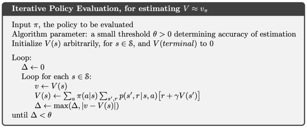
Iterative Policy Evaluation

In RL, policy evaluation is referred to as a prediction problem. A prediction problem asks, given a known policy $\pi$ , what is its state-value function $v_\pi(s)$ ?

Iterative Policy Evaluation is a prediction method within Dynamic Programming. It uses the Bellman equation as its update rule. Under the same conditions that guarantee the existence of $v_\pi$ , the sequence $\{ v_k \}$ converges to $v_\pi$ as $k \rightarrow \infty$ .

$\displaystyle v_{k+1} \doteq \mathbb{E}_\pi \left[ R_{t+1} + \gamma v_k(S_{t+1}) \mid S_t=s \right] \\\\ \hphantom{v_{k+1}} = \sum_a \pi(a \mid s) \sum_{s^\prime, r} p(s^\prime, r \mid s, a) \left[ r + \gamma v_k(s^\prime) \right]$

The algorithm for iterative policy evaluation is as follows:

Iterative Policy Evaluation (source: Reinforcement Learning: An Introduction, 2nd).

Control

In RL, the goal of a control problem is to find an optimal policy $\pi_*$ by repeatedly performing policy evaluation and policy improvement, such that the expected return is maximized for all states.

Next, we introduce two control methods in Dynamic Programming.

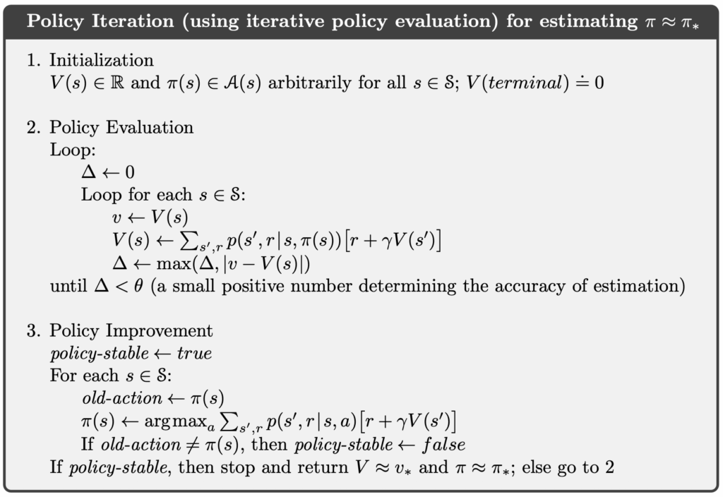
Policy Iteration

The idea of policy iteration in DP is that once a policy $\pi$ is improved using its state-value function $v_\pi$ , yielding a better policy $\pi^\prime$ , we can then evaluate $v_{\pi^\prime}$ and obtain a further improved policy $\pi^{\prime\prime}$ . Since a finite MDP has only a finite number of policies, this process is guaranteed to eventually converge to the optimal policy and the optimal state-value function.

The algorithm for policy iteration is as follows:

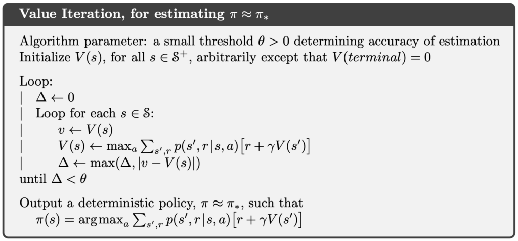
Policy Iteration (source: Reinforcement Learning: An Introduction, 2nd).

Value Iteration

One drawback of policy iteration is that each iteration involves policy evaluation, which requires multiple iterative updates over all states and can therefore be computationally expensive.

Value Iteration addresses this issue by combining policy evaluation and policy improvement into a single step, using the Bellman optimality equation for updates. For any initial value function $v_0$ , under the same conditions that guarantee the existence of the optimal value function $v_*$ , the sequence $\{ v_k \}$ can be shown to converge to $v_*$ .

$\displaystyle v_{k+1} \doteq \max_a \mathbb{E} \left[ R_{t+1} + \gamma v_k(S_{t+1}) \mid S_t=s \right] \\\\ \hphantom{v_{k+1}} = \max_a \sum_{s^\prime, r} p(s^\prime, r \mid s, a) \left[ r + \gamma v_k(s^\prime) \right]$

Once $v_k$ has sufficiently converged, the optimal policy $\pi_*$ is given by:

$\displaystyle \pi_*(s) = \text{argmax}_a \sum_{s^\prime, r} p(s^\prime, r \mid s, a) \left[ r + \gamma v_k(s^\prime) \right]$

The algorithm for value iteration is as follows:

Value Iteration (source: Reinforcement Learning: An Introduction, 2nd).

Efficiency and Limitations

DP directly uses the Bellman equations and requires no sampling, resulting in no estimation error. As a result, its convergence process is stable and predictable. However, the limitations of DP are severe, making it almost impossible to apply in practical RL settings. The main reasons are:

It requires a complete environment model.
It requires full sweeps over all states, leading to a very high computational cost.
It cannot handle continuous or high-dimensional state spaces.

Although DP cannot be applied to large-scale problems, it remains an indispensable component of RL because it provides the conceptual foundation for all other methods. The Bellman equations in their DP form underpin every other RL algorithm.

Examples

Implementation

In the following code, we faithfully implement the two control methods of DP, policy iteration and value iteration.

The variable env is a Gymnasium Env object. Gymnasium is the successor to OpenAI Gym and provides a wide range of RL environments, allowing us to test reinforcement learning algorithms in simulated settings.

An environment contains env.observation_space.n states. Accordingly, states are indexed by integers from 0 to env.observation_space.n - 1. The variable V is a one-dimensional array of floating-point values, where each element represents the estimated state-value of a state. For example, V[0] is the estimated state-value of state 0.

Each state has env.action_space.n possible actions, indexed from 0 to env.action_space.n - 1. The policy pi is a two-dimensional floating-point array of shape [env.observation_space.n][env.action_space.n]. Each entry pi[s][a] is a probability in the range $\left[ 0,1 \right]$ , and for each state $s$ , the probabilities over all actions sum to 1.

The environment’s env.unwrapped.P represents the transition dynamics. Each entry env.unwrapped.P[s][a] contains the next state, the reward, the transition probability, and an indicator of whether the next state is terminal.

class DynamicProgramming:
    def __init__(self, env: gym.Env, gamma=0.9, theta=1e-9):
        self.env = env
        self.gamma = gamma
        self.theta = theta

    def _policy_evaluation(self, pi: np.ndarray, V: np.ndarray) -> np.ndarray:
        while True:
            delta = 0
            for s in range(self.env.observation_space.n):
                v = 0
                for a, pi_as in enumerate(pi[s]):
                    q_sa = 0
                    for p, s_prime, r, terminated in self.env.unwrapped.P[s][a]:
                        q_sa += p * (r + self.gamma * V[s_prime] * (not terminated))
                    v += pi_as * q_sa
                delta = max(delta, np.abs(v - V[s]))
                V[s] = v

            if delta < self.theta:
                break

        return V

    def _policy_improvement(self, pi: np.ndarray, V: np.ndarray) -> tuple[np.ndarray, bool]:
        policy_stable = True

        for s in range(self.env.observation_space.n):
            old_a = np.argmax(pi[s])
            pi[s] = self._greedify_policy(V, s)
            new_a = np.argmax(pi[s])

            if old_a != new_a:
                policy_stable = False

        return pi, policy_stable

    def _greedify_policy(self, V: np.ndarray, s: int) -> np.ndarray:
        q_s = np.zeros(self.env.action_space.n)
        for a in range(self.env.action_space.n):
            for p, s_prime, r, terminated in self.env.unwrapped.P[s][a]:
                q_s[a] += p * (r + self.gamma * V[s_prime] * (not terminated))

        new_a = np.argmax(q_s)
        pi_s = np.eye(self.env.action_space.n)[new_a]
        return pi_s

    def policy_iteration(self) -> tuple[np.ndarray, np.ndarray]:
        V = np.zeros(self.env.observation_space.n)
        pi = np.ones((self.env.observation_space.n, self.env.action_space.n)) / self.env.action_space.n
        policy_stable = False

        while not policy_stable:
            V = self._policy_evaluation(pi, V)
            pi, policy_stable = self._policy_improvement(pi, V)

        return pi, V

    def value_iteration(self) -> tuple[np.ndarray, np.ndarray]:
        V = np.zeros(self.env.observation_space.n)

        while True:
            delta = 0
            for s in range(self.env.observation_space.n):
                q_s = np.zeros(self.env.action_space.n)
                for a in range(self.env.action_space.n):
                    for p, s_prime, r, terminated in self.env.unwrapped.P[s][a]:
                        q_s[a] += p * (r + self.gamma * V[s_prime] * (not terminated))

                new_a = np.max(q_s)
                delta = max(delta, np.abs(new_a - V[s]))
                V[s] = new_a

            if delta < self.theta:
                break

        pi = np.zeros((self.env.observation_space.n, self.env.action_space.n))
        for s in range(self.env.observation_space.n):
            pi[s] = self._greedify_policy(V, s)

        return pi, V

Cliff Walking

Cliff Walking involves moving from a start position to a goal position in a grid world while avoiding falling off a cliff, as illustrated below.

In the Cliff Walking problem, each state corresponds to the player’s current position. There are a total of 36 states, consisting of the top three rows plus the bottom-left cell, giving $3 \times 12 + 1 = 36$ states. The current position is computed using the following formula:

$\text{position} = \text{current-row} \times \text{num-col} + \text{current-col}$

There are four available actions:

0: Move up
1: Move right
2: Move down
3: Move left

Each step yields a reward of −1. However, if the agent steps into the cliff, it receives a reward of −100.

import time

import gymnasium as gym
import numpy as np

from dp import DynamicProgramming

GYM_ID = "CliffWalking-v1"


def play_game(policy, episodes=1):
    visual_env = gym.make(GYM_ID, render_mode="human")

    for episode in range(episodes):
        state, _ = visual_env.reset()
        terminated = False
        truncated = False
        total_reward = 0
        step_count = 0

        print(f"Episode {episode + 1} starts")
        while not terminated and not truncated:
            action = np.argmax(policy[state])
            state, reward, terminated, truncated, _ = visual_env.step(action)
            total_reward += reward
            step_count += 1
            time.sleep(0.3)

        print(f"Episode {episode + 1} is finished: Total reward is {total_reward}, steps = {step_count}")
        time.sleep(1)

    visual_env.close()


if __name__ == "__main__":
    env = gym.make(GYM_ID)
    dp = DynamicProgramming(env)

    print(f"Gym environment: {GYM_ID}")

    print("Start DP Policy Iteration")
    pi_policy, pi_V = dp.policy_iteration()
    play_game(pi_policy)

    print("\n")

    print("Start DP Value Iteration")
    vi_policy, vi_V = dp.value_iteration()
    play_game(vi_policy)

    env.close()

The following figure shows the execution result of the above program. After training, the agent learns a policy that moves along the edge of the cliff and reaches the goal through the shortest path, which corresponds to the optimal behavior in the Cliff Walking environment under the given reward structure.

Taxi

The Taxi problem takes place in a grid world where the agent must navigate to the passenger’s location, pick up the passenger, and then deliver them to one of four designated destinations, as illustrated below.

In the Taxi problem, there are 500 discrete states. Each state is encoded by the following formula:

$r: \text{the row the taxi is currently at} \\\\ c: \text{the colunm the taxi is currently at} \\\\ p: \text{the location the passenger is at} \\\\ d: \text{the destination to drop off the passenger} \\\\ state = ((r \times 5 + c) \times 5 + p) * 4 + d$

Passenger locations are defined as:

0: Red
1: Green
2: Yellow
3: Blue
4: In taxi

Destinations are defined as:

0: Red
1: Green
2: Yellow
3: Blue

There are six available actions:

0: Move south (down)
1: Move north (up)
2: Move east (right)
3: Move west (left)
4: Pick up passenger
5: Drop off passenger

Each step yields a reward of −1 unless another reward is triggered. Successfully delivering the passenger to the destination yields a reward of +20. Executing an illegal pickup or drop-off action results in a reward of −10.

import time

import gymnasium as gym
import numpy as np

from dp import DynamicProgramming

GYM_ID = "Taxi-v3"


def play_game(policy, episodes=1):
    visual_env = gym.make(GYM_ID, render_mode="human")

    for episode in range(episodes):
        state, _ = visual_env.reset()
        terminated = False
        truncated = False
        total_reward = 0
        step_count = 0

        print(f"Episode {episode + 1} starts")
        while not terminated and not truncated:
            action = np.argmax(policy[state])
            state, reward, terminated, truncated, _ = visual_env.step(action)
            total_reward += reward
            step_count += 1
            time.sleep(0.3)

        print(f"Episode {episode + 1} is finished: Total reward is {total_reward}, steps = {step_count}")
        time.sleep(1)

    visual_env.close()


if __name__ == "__main__":
    env = gym.make(GYM_ID)
    dp = DynamicProgramming(env)

    print(f"Gym environment: {GYM_ID}")

    print("Start DP Policy Iteration")
    pi_policy, pi_V = dp.policy_iteration()
    play_game(pi_policy)

    print("\n")

    print("Start DP Value Iteration")
    vi_policy, vi_V = dp.value_iteration()
    play_game(vi_policy)

    env.close()

Below are the execution results of the above program.

Conclusion

DP, through explicit Bellman equations, complete model information, and systematic sweeps, provides the purest and most mathematically grounded approach to policy evaluation and policy improvement. Although DP requires a complete environment model and exhaustive traversal of the entire state space, making it impractical for direct application in complex real-world environments—its value lies not in implementation, but in the conceptual foundation it establishes. Consequently, even though DP itself is unsuitable for large-scale problems, it remains the basis for understanding all subsequent RL algorithms.

References

Adam White and Martha White. Reinforcement Learning Specialization. University of Alberta and Coursera.
Richard S. Sutton and Andrew G. Barto. 2020. Reinforcement Learning: An Introduction, 2^nd. The MIT Press.

Dynamic Programming, DP

Share

Table of Contents

Reinforcement Learning Method Classification

Model-Based vs. Model-Free

Bootstrapping vs. Non-Bootstrapping

On-Policy vs. Off-Policy

Dynamic Programming, DP

Prediction

Iterative Policy Evaluation

Control

Policy Iteration

Value Iteration

Efficiency and Limitations

Examples

Implementation

Cliff Walking

Taxi

Conclusion

References

Related Tags

Leave a Reply Cancel reply

You May Also Like