
A Markov Decision Process (MDP) provides the rigorous mathematical foundation underlying all policy evaluation and policy improvement methods in Reinforcement Learning (RL). Through an MDP, we can formally describe the interaction between an agent and its environment, and define the value of a policy in terms of its expected return.
Table of Contents
Markov Decision Process (MDP)
A Markov Decision Process (MDP) is a model for sequential decision-making in situations where outcomes are uncertain. Originating in operations research in the 1950s, the MDP framework has since become influential across many fields. Its name reflects its connection to Markov chains, introduced by the Russian mathematician Andrey Markov.
An MDP is the formal mathematical model of reinforcement learning. It provides a simple yet expressive framework for learning from interactions to achieve a goal. These interactions refer to the continual exchange between an agent and its environment, as illustrated below.
The agent and the environment interact over a sequence of time steps,  . At each time step
  , the agent receives a state representation from the environment,
  . Based on this state, the agent selects an action,
  . At the next time step
  , the agent receives a reward,
  , and simultaneously observes its new state
  .
.
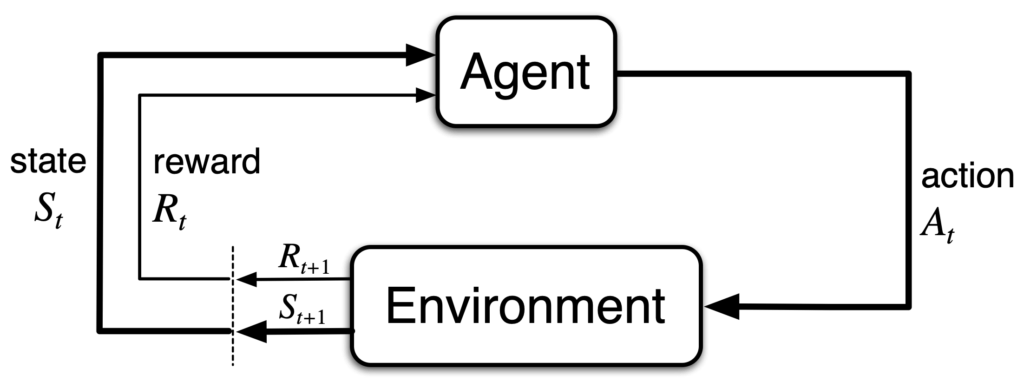
Thus, the MDP together with the agent generates a trajectory of the following form:

A complete MDP is defined by the following five components:

State Space
The state space, denoted by  , represents all possible states. At each time step , the agent occupies some state . The current state
  contains all information observable to the agent at time step , and is used to determine the next action
  . Therefore, the state must include all features of past agent–environment interactions that may influence future outcomes. When this condition is satisfied, the state is said to possess the Markov property:

In other words, when the agent is in state , it can discard all previous states and actions, ( ). The future depends only on the present, not the past.
Action Space
The action space, denoted by  , defines the set of actions available to the agent.
For each state  , the set of allowable actions is denoted by
  .
.
State-Transition Probabilities
After choosing an action  in state , the environment may transition to various possible next states. This is governed by the state-transition dynamics
  , which determine the next state
  and reward
  .
.
![\displaystyle p(s^\prime, r \mid s, a) \doteq \Pr\{S_t=s^\prime, R_t=r \mid S_{t-1}=s, A_{t-1}=a\} \\\\ \sum_{s^\prime \in \mathcal{S}} \sum_{r \in \mathcal{R}} p(s^\prime, r \mid s, a) = 1, \forall s \in \mathcal{S}, a \in \mathcal{A}(s) \\\\ p(s^\prime \mid s, a) \doteq \mathbb{E} \left[ R_t \mid S_{t-1}=s, A_{t-1}=a \right] = \sum_{r \in \mathcal{R}} p(s^\prime, r \mid s, a)](https://s0.wp.com/latex.php?latex=%5Cdisplaystyle+p%28s%5E%5Cprime%2C+r+%5Cmid+s%2C+a%29+%5Cdoteq+%5CPr%5C%7BS_t%3Ds%5E%5Cprime%2C+R_t%3Dr+%5Cmid+S_%7Bt-1%7D%3Ds%2C+A_%7Bt-1%7D%3Da%5C%7D+%5C%5C%5C%5C+%5Csum_%7Bs%5E%5Cprime+%5Cin+%5Cmathcal%7BS%7D%7D+%5Csum_%7Br+%5Cin+%5Cmathcal%7BR%7D%7D+p%28s%5E%5Cprime%2C+r+%5Cmid+s%2C+a%29+%3D+1%2C+%5Cforall+s+%5Cin+%5Cmathcal%7BS%7D%2C+a+%5Cin+%5Cmathcal%7BA%7D%28s%29+%5C%5C%5C%5C+p%28s%5E%5Cprime+%5Cmid+s%2C+a%29+%5Cdoteq+%5Cmathbb%7BE%7D+%5Cleft%5B+R_t+%5Cmid+S_%7Bt-1%7D%3Ds%2C+A_%7Bt-1%7D%3Da+%5Cright%5D+%3D+%5Csum_%7Br+%5Cin+%5Cmathcal%7BR%7D%7D+p%28s%5E%5Cprime%2C+r+%5Cmid+s%2C+a%29+&bg=ffffff&fg=000&s=1&c=20201002)
Reward
The reward, denoted by  , represents the immediate feedback received. A reward is produced when the agent takes action a in state s and transitions to a new state .
![\displaystyle r(s, a, s^\prime) \doteq \mathbb{E} \left[ R_t \mid S_{t-1}=s, A_{t-1}=a, S_t=s^\prime \right] = \sum_{r \in \mathcal{R}} r \frac{p(s^\prime, r \mid s, a)}{p(s^\prime \mid s, a)} \\\\ r(s, a) \doteq \mathbb{E} \left[ R_t \mid S_{t-1}=s, A_{t-1}=a \right] = \sum_{r \in \mathcal{R}} r \sum_{s^\prime \in \mathcal{S}} p(s^\prime, r \mid s, a)](https://s0.wp.com/latex.php?latex=%5Cdisplaystyle+r%28s%2C+a%2C+s%5E%5Cprime%29+%5Cdoteq+%5Cmathbb%7BE%7D+%5Cleft%5B+R_t+%5Cmid+S_%7Bt-1%7D%3Ds%2C+A_%7Bt-1%7D%3Da%2C+S_t%3Ds%5E%5Cprime+%5Cright%5D+%3D+%5Csum_%7Br+%5Cin+%5Cmathcal%7BR%7D%7D+r+%5Cfrac%7Bp%28s%5E%5Cprime%2C+r+%5Cmid+s%2C+a%29%7D%7Bp%28s%5E%5Cprime+%5Cmid+s%2C+a%29%7D+%5C%5C%5C%5C+r%28s%2C+a%29+%5Cdoteq+%5Cmathbb%7BE%7D+%5Cleft%5B+R_t+%5Cmid+S_%7Bt-1%7D%3Ds%2C+A_%7Bt-1%7D%3Da+%5Cright%5D+%3D+%5Csum_%7Br+%5Cin+%5Cmathcal%7BR%7D%7D+r+%5Csum_%7Bs%5E%5Cprime+%5Cin+%5Cmathcal%7BS%7D%7D+p%28s%5E%5Cprime%2C+r+%5Cmid+s%2C+a%29+&bg=ffffff&fg=000&s=1&c=20201002)
Discount Factor
The discount factor, denoted ![\gamma \in \left[ 0,1 \right]](https://s0.wp.com/latex.php?latex=%5Cgamma+%5Cin+%5Cleft%5B+0%2C1+%5Cright%5D&bg=ffffff&fg=000&s=0&c=20201002) , quantifies how much future rewards are valued. When
, quantifies how much future rewards are valued. When  , only immediate rewards matter; when
  , all future rewards are valued equally with present rewards.
Returns and Episodes
The agent’s long-term objective is to maximize the cumulative reward. It aims to maximize the expected return. The return at time step , denoted  , in the simplest case is the sum of future rewards:

where  is the final time step.
When the interaction between the agent and the environment naturally breaks into subsequences, each subsequence is called an episode. Every episode ends in a special state known as a terminal state, and episodes are independent of one another. Such tasks are referred to as episodic tasks, as in the case of a single game.
When the interaction does not naturally break into episodes and continues indefinitely, the task is referred to as a continuing task, such as in long-lived robotic applications. In such cases, the final time step becomes  in the expression for . Without additional structure, maximizing the return would cause to diverge.
To address this issue, we apply discounting. The agent instead maximizes the expected discounted return:

where is the discount factor.
Returns from successive time steps are closely related, a property that is crucial in RL theory and algorithms::

Although the discounted return consists of infinitely many terms, it remains finite as long as the reward is bounded and  . For example, if the reward is constantly
  , then:

Policy
A policy, denoted  , specifies how the agent selects an action from the action set available in each state . Formally, a policy is a probability distribution over actions conditioned on the current state.
At time step , when the agent is in state , the probability that it chooses action a according to policy is:

A policy may be deterministic, meaning the policy always selects a single specific action:

A policy may also be stochastic, in which case each available action has some probability of being selected.
Value Function
A value function evaluates a policy by estimating the expected return an agent can obtain when following that policy. In other words, under a policy , the value function quantifies how much cumulative reward the agent can expect in the future.
State-Value Function
Under policy , the state-value function measures the expected return when starting from state . It is denoted by  :
:
![\displaystyle v_\pi(s) \doteq \mathbb{E}_\pi \left[ G_t \mid S_t=s \right] = \mathbb{E}_\pi \left[ \sum_{k=0}^\infty \gamma^k R_{t+k+1} \mid S_t=s \right], \forall s \in \mathcal{S}](https://s0.wp.com/latex.php?latex=%5Cdisplaystyle+v_%5Cpi%28s%29+%5Cdoteq+%5Cmathbb%7BE%7D_%5Cpi+%5Cleft%5B+G_t+%5Cmid+S_t%3Ds+%5Cright%5D+%3D+%5Cmathbb%7BE%7D_%5Cpi+%5Cleft%5B+%5Csum_%7Bk%3D0%7D%5E%5Cinfty+%5Cgamma%5Ek+R_%7Bt%2Bk%2B1%7D+%5Cmid+S_t%3Ds+%5Cright%5D%2C+%5Cforall+s+%5Cin+%5Cmathcal%7BS%7D+&bg=ffffff&fg=000&s=1&c=20201002)
Action-Value Function
Under policy , the action-value function measures the expected return when starting from state s and taking action . It is denoted by  , commonly referred to as the q-function:
![\displaystyle q_\pi(s,a) \doteq \mathbb{E}_\pi \left[ G_t \mid S_t=s, A_t=a \right] = \mathbb{E}_\pi \left[ \sum_{k=0}^\infty \gamma^k R_{t+k+1} \mid S_t=s, A_t=a \right]](https://s0.wp.com/latex.php?latex=%5Cdisplaystyle+q_%5Cpi%28s%2Ca%29+%5Cdoteq+%5Cmathbb%7BE%7D_%5Cpi+%5Cleft%5B+G_t+%5Cmid+S_t%3Ds%2C+A_t%3Da+%5Cright%5D+%3D+%5Cmathbb%7BE%7D_%5Cpi+%5Cleft%5B+%5Csum_%7Bk%3D0%7D%5E%5Cinfty+%5Cgamma%5Ek+R_%7Bt%2Bk%2B1%7D+%5Cmid+S_t%3Ds%2C+A_t%3Da+%5Cright%5D+&bg=ffffff&fg=000&s=1&c=20201002)
Relationship Between State-Value Function and Action-Value Function
The relationship between the state-value function  and the action-value function
  is fundamental throughout reinforcement learning. The formulas in this section will appear repeatedly across RL algorithms.
Below is the backup diagram for  , where hollow circles represent states and solid circles represent actions. This diagram summarizes all elements discussed so far. In state , an action is selected according to policy . Then, according to the state-transition probabilities , the next state is determined and a reward is generated for reaching .
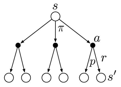
First, consider the relationship from the state-value function to the action-value function. In a given state , the value is the expectation over all possible actions weighted by the policy  . In other words, the state-value function can be viewed as the expectation of the action-value function.

Next, consider the recursive relationship from the action-value function back to the state-value function. After taking action in state , the value is the expectation over all possible next states and corresponding rewards , weighted by the state-transition probabilities  . For each possible pair
  , we sum the immediate reward and the discounted future value
  . Thus, the action-value function equals the immediate reward plus the discounted expectation of the state-value function.
![\displaystyle q_\pi(s, a) = \sum_{s^\prime, r} p(s^\prime, r \mid s, a) \left[ r + \gamma v_\pi(s^\prime) \right]](https://s0.wp.com/latex.php?latex=%5Cdisplaystyle+q_%5Cpi%28s%2C+a%29+%3D+%5Csum_%7Bs%5E%5Cprime%2C+r%7D+p%28s%5E%5Cprime%2C+r+%5Cmid+s%2C+a%29+%5Cleft%5B+r+%2B+%5Cgamma+v_%5Cpi%28s%5E%5Cprime%29+%5Cright%5D+&bg=ffffff&fg=000&s=1&c=20201002)
Bellman Expectation Equation
The Bellman Equation, named after Richard E. Bellman, is a fundamental technique in Dynamic Programming. Bellman’s principle of optimality states that an optimization problem can be decomposed into a recursive structure of subproblems. The value of any state can be expressed as the immediate reward resulting from an initial choice plus the value of the subsequent subproblem induced by that choice.
Therefore, the essential idea of the Bellman equation is that the value of a state can be written as the expected immediate reward plus the expected value of the next state.
Bellman Expectation Equation for State-Value Function
Under a policy , the state-value function can be written recursively as:
![\displaystyle v_\pi(s) \doteq \mathbb{E}_\pi \left[ G_t \mid S_t=s \right] \\\\ \hphantom{v_\pi(s)} = \mathbb{E}_\pi \left[ R_{t+1} + \gamma G_{t+1} \mid S_t=s \right] \\\\ \hphantom{v_\pi(s)} = \sum_a \pi(a \mid s) \sum_{s^\prime} \sum_r p(s^\prime, r \mid s, a) \Big[ r + \gamma \mathbb{E}_\pi \left[ G_{t+1} \mid S_{t+1} = s^\prime \right] \Big] \\\\ \hphantom{v_\pi(s)} = \sum_a \pi(a \mid s) \sum_{s^\prime} \sum_r p(s^\prime, r \mid s, a) \Big[ r + \gamma v_\pi(s^\prime) \Big], \forall s \in \mathcal{S}](https://s0.wp.com/latex.php?latex=%5Cdisplaystyle+v_%5Cpi%28s%29+%5Cdoteq+%5Cmathbb%7BE%7D_%5Cpi+%5Cleft%5B+G_t+%5Cmid+S_t%3Ds+%5Cright%5D+%5C%5C%5C%5C+%5Chphantom%7Bv_%5Cpi%28s%29%7D+%3D+%5Cmathbb%7BE%7D_%5Cpi+%5Cleft%5B+R_%7Bt%2B1%7D+%2B+%5Cgamma+G_%7Bt%2B1%7D+%5Cmid+S_t%3Ds+%5Cright%5D+%5C%5C%5C%5C+%5Chphantom%7Bv_%5Cpi%28s%29%7D+%3D+%5Csum_a+%5Cpi%28a+%5Cmid+s%29+%5Csum_%7Bs%5E%5Cprime%7D+%5Csum_r+p%28s%5E%5Cprime%2C+r+%5Cmid+s%2C+a%29+%5CBig%5B+r+%2B+%5Cgamma+%5Cmathbb%7BE%7D_%5Cpi+%5Cleft%5B+G_%7Bt%2B1%7D+%5Cmid+S_%7Bt%2B1%7D+%3D+s%5E%5Cprime+%5Cright%5D+%5CBig%5D+%5C%5C%5C%5C+%5Chphantom%7Bv_%5Cpi%28s%29%7D+%3D+%5Csum_a+%5Cpi%28a+%5Cmid+s%29+%5Csum_%7Bs%5E%5Cprime%7D+%5Csum_r+p%28s%5E%5Cprime%2C+r+%5Cmid+s%2C+a%29+%5CBig%5B+r+%2B+%5Cgamma+v_%5Cpi%28s%5E%5Cprime%29+%5CBig%5D%2C+%5Cforall+s+%5Cin+%5Cmathcal%7BS%7D+&bg=ffffff&fg=000&s=1&c=20201002)
This equation states that the value is the expectation over all possible actions weighted by the policy . Each action’s value is, in turn, the expected immediate reward plus the discounted value of the next state, weighted by the transition probabilities . For this reason, the equation is known as the Bellman Expectation Equation.
Bellman Expectation Equation for Action-Value Function
Applying the same recursive reasoning to the action-value function  yields:
![\displaystyle q_\pi(s, a) \doteq \mathbb{E}_\pi \left[ G_t \mid S_t=s, A_t=a \right] \\\\ \hphantom{v_\pi(s, a)} = \mathbb{E}_\pi \left[ R_{t+1} + \gamma G_{t+1} \mid S_t=s, A_t=a \right] \\\\ \hphantom{v_\pi(s, a)} = \sum_{s^\prime} \sum_r p(s^\prime, r \mid s, a) \Big[ r + \gamma \mathbb{E}_\pi \left[ G_{t+1} \mid S_{t+1} = s^\prime \right] \Big] \\\\ \hphantom{v_\pi(s, a)} = \sum_{s^\prime} \sum_r p(s^\prime, r \mid s, a) \Big[ r + \gamma v_\pi(s^\prime) \Big], \forall s \in \mathcal{S}, a \in \mathcal{A}(s)](https://s0.wp.com/latex.php?latex=%5Cdisplaystyle+q_%5Cpi%28s%2C+a%29+%5Cdoteq+%5Cmathbb%7BE%7D_%5Cpi+%5Cleft%5B+G_t+%5Cmid+S_t%3Ds%2C+A_t%3Da+%5Cright%5D+%5C%5C%5C%5C+%5Chphantom%7Bv_%5Cpi%28s%2C+a%29%7D+%3D+%5Cmathbb%7BE%7D_%5Cpi+%5Cleft%5B+R_%7Bt%2B1%7D+%2B+%5Cgamma+G_%7Bt%2B1%7D+%5Cmid+S_t%3Ds%2C+A_t%3Da+%5Cright%5D+%5C%5C%5C%5C+%5Chphantom%7Bv_%5Cpi%28s%2C+a%29%7D+%3D+%5Csum_%7Bs%5E%5Cprime%7D+%5Csum_r+p%28s%5E%5Cprime%2C+r+%5Cmid+s%2C+a%29+%5CBig%5B+r+%2B+%5Cgamma+%5Cmathbb%7BE%7D_%5Cpi+%5Cleft%5B+G_%7Bt%2B1%7D+%5Cmid+S_%7Bt%2B1%7D+%3D+s%5E%5Cprime+%5Cright%5D+%5CBig%5D+%5C%5C%5C%5C+%5Chphantom%7Bv_%5Cpi%28s%2C+a%29%7D+%3D+%5Csum_%7Bs%5E%5Cprime%7D+%5Csum_r+p%28s%5E%5Cprime%2C+r+%5Cmid+s%2C+a%29+%5CBig%5B+r+%2B+%5Cgamma+v_%5Cpi%28s%5E%5Cprime%29+%5CBig%5D%2C+%5Cforall+s+%5Cin+%5Cmathcal%7BS%7D%2C+a+%5Cin+%5Cmathcal%7BA%7D%28s%29+&bg=ffffff&fg=000&s=1&c=20201002)
This equation describes the value of taking action in state as the expectation over the immediate reward and the discounted future state-value, weighted by the environment’s transition probabilities .
Optimal Policy
Solving a reinforcement learning task means discovering a policy that achieves high cumulative reward over the long run. For a finite MDP, an optimal policy can be defined precisely. Value functions impose a partial ordering over policies: if, for every state, the expected return of one policy is greater than or equal to that of another policy  , then policy is said to be better than or equal to .

There always exists at least one policy that is better than or equal to all other policies. Such a policy is called an optimal policy. Although there may be multiple optimal policies, we denote the entire set of them by  .
.
All optimal policies share the same optimal state-value function, denoted  :
:

They also share the same optimal action-value function, denoted  .
.

Bellman Optimality Equation
Bellman Optimality Equation for Optimal State-Value Function
Under an optimal policy , the optimal state-value function can be written in the following recursive form:
![\displaystyle v_*(s)=\max_{a \in \mathcal{A}(s)} q_* (s, a) \\\\ \hphantom{v_*(s)} = \max_a \mathbb{E}_{\pi_*} \left[ G_t \mid S_t=s, A_t=a \right] \\\\ \hphantom{v_*(s)} = \max_a \mathbb{E}_{\pi_*} \left[ R_{t+1} + \gamma G_{t+1} \mid S_t=s, A_t=a \right] \\\\ \hphantom{v_*(s)} = \max_a \mathbb{E} \left[ R_{t+1} + \gamma v_*(S_{t+1}) \mid S_t=s, A_t=a \right] \\\\ \hphantom{v_*(s)} = \max_a \sum_{s^\prime, r} p(s^\prime, r \mid s, a) \left[ r + \gamma v_*(s^\prime) \right]](https://s0.wp.com/latex.php?latex=%5Cdisplaystyle+v_%2A%28s%29%3D%5Cmax_%7Ba+%5Cin+%5Cmathcal%7BA%7D%28s%29%7D+q_%2A+%28s%2C+a%29+%5C%5C%5C%5C+%5Chphantom%7Bv_%2A%28s%29%7D+%3D+%5Cmax_a+%5Cmathbb%7BE%7D_%7B%5Cpi_%2A%7D+%5Cleft%5B+G_t+%5Cmid+S_t%3Ds%2C+A_t%3Da+%5Cright%5D+%5C%5C%5C%5C+%5Chphantom%7Bv_%2A%28s%29%7D+%3D+%5Cmax_a+%5Cmathbb%7BE%7D_%7B%5Cpi_%2A%7D+%5Cleft%5B+R_%7Bt%2B1%7D+%2B+%5Cgamma+G_%7Bt%2B1%7D+%5Cmid+S_t%3Ds%2C+A_t%3Da+%5Cright%5D+%5C%5C%5C%5C+%5Chphantom%7Bv_%2A%28s%29%7D+%3D+%5Cmax_a+%5Cmathbb%7BE%7D+%5Cleft%5B+R_%7Bt%2B1%7D+%2B+%5Cgamma+v_%2A%28S_%7Bt%2B1%7D%29+%5Cmid+S_t%3Ds%2C+A_t%3Da+%5Cright%5D+%5C%5C%5C%5C+%5Chphantom%7Bv_%2A%28s%29%7D+%3D+%5Cmax_a+%5Csum_%7Bs%5E%5Cprime%2C+r%7D+p%28s%5E%5Cprime%2C+r+%5Cmid+s%2C+a%29+%5Cleft%5B+r+%2B+%5Cgamma+v_%2A%28s%5E%5Cprime%29+%5Cright%5D+&bg=ffffff&fg=000&s=1&c=20201002)
Here, the operator  indicates that, in each state, the agent chooses the action that maximizes the expected value. This captures the essence of an optimal policy. This recursive relationship is the Bellman Optimality Equation for .
Bellman Optimality Equation for Optimal Action-Value Function
Under an optimal policy , the optimal action-value function satisfies the following recursive form:
![\displaystyle q_*(s, a) = \mathbb{E} \left[ R_{t+1} + \gamma \max_{a^\prime} q_*(S_{t+1}, a^\prime) \mid S_t=s, A_t=a \right] \\\\ \hphantom{q_*(s, a)} = \sum_{s^\prime, r} p(s^\prime, r \mid s, a) \left[ r + \gamma \max_{a^\prime} q_*(s^\prime, a^\prime) \right]](https://s0.wp.com/latex.php?latex=%5Cdisplaystyle+q_%2A%28s%2C+a%29+%3D+%5Cmathbb%7BE%7D+%5Cleft%5B+R_%7Bt%2B1%7D+%2B+%5Cgamma+%5Cmax_%7Ba%5E%5Cprime%7D+q_%2A%28S_%7Bt%2B1%7D%2C+a%5E%5Cprime%29+%5Cmid+S_t%3Ds%2C+A_t%3Da+%5Cright%5D+%5C%5C%5C%5C+%5Chphantom%7Bq_%2A%28s%2C+a%29%7D+%3D+%5Csum_%7Bs%5E%5Cprime%2C+r%7D+p%28s%5E%5Cprime%2C+r+%5Cmid+s%2C+a%29+%5Cleft%5B+r+%2B+%5Cgamma+%5Cmax_%7Ba%5E%5Cprime%7D+q_%2A%28s%5E%5Cprime%2C+a%5E%5Cprime%29+%5Cright%5D+&bg=ffffff&fg=000&s=1&c=20201002)
This expression is the Bellman Optimality Equation for .
Conclusion
The MDP framework provides a precise and operational mathematical description for decision-making problems in reinforcement learning. It enables us to define policies, evaluate their long-term performance, and compare the quality of different policies. All subsequent control methods and optimal policy–search techniques ultimately trace back to this foundational set of definitions established by the MDP framework.
References
- Adam White and Martha White. Reinforcement Learning Specialization. University of Alberta and Coursera.
- Richard S. Sutton and Andrew G. Barto. 2020. Reinforcement Learning: An Introduction, 2nd. The MIT Press.


