
In the field of image recognition, Convolutional Neural Networks (CNNs) have long been the dominant architecture. In recent years, Transformer models have achieved great success in Natural Language Processing (NLP), which has led researchers to consider applying the Transformer architecture to image processing tasks. Vision Transformer (ViT) is a model designed for image understanding based on the Transformer framework.
The complete code for this chapter can be found in .
Table of Contents
Vision Transformer (ViT) Architecture
Vision Transformer (ViT) was proposed by Google Research in 2020. It builds upon the success of the Transformer architecture in NLP and extends its application to the visual domain. Although CNNs have demonstrated strong performance in image processing, their core design is inherently local, which limits their ability to model long-range dependencies. ViT aims to leverage the global attention mechanism of Transformers to capture relationships between distant regions in an image, thereby improving recognition performance. However, since Transformers were originally designed for token sequences in text, the first challenge ViT must address is how to convert an image into a sequential format suitable for Transformer input.
The overall structure of ViT is based on the encoder part of the Transformer. If you are not yet familiar with Transformers, it is recommended to refer to the following article first.

The authors of ViT sought to use the original Transformer design with minimal modifications. However, because traditional Transformers accept token sequences as input, an image must first be transformed into a format compatible with this requirement.
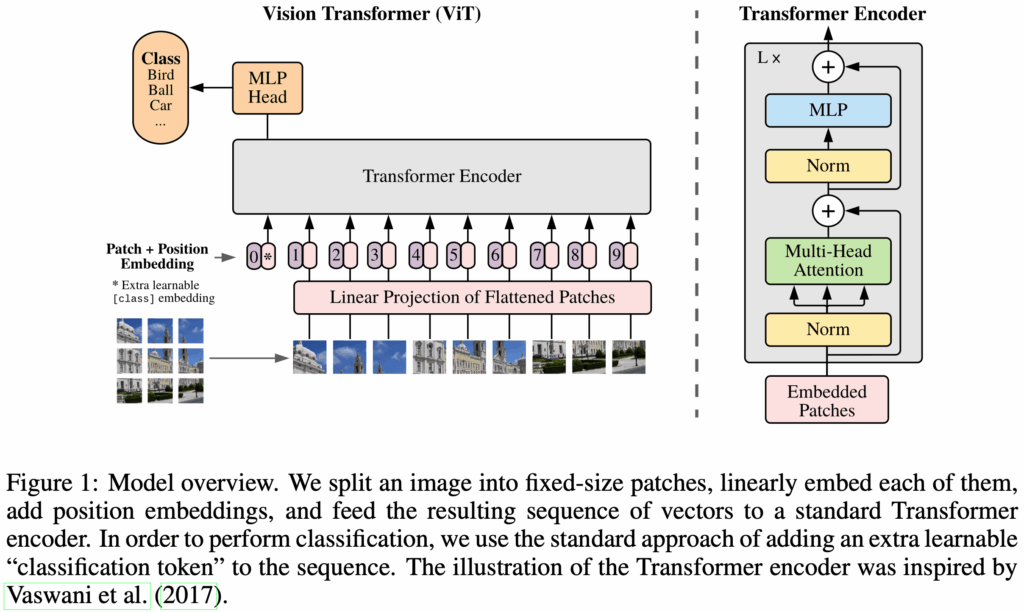
The following figure shows an overview of the ViT model.
Patch Embeddings
The input image is denoted as  , where
  is the image height,
  is the width, and
  is the number of channels (e.g., 3 for RGB). The image
  is split into non-overlapping patches of size
  . Each patch, therefore, has shape
  . Each patch is then flattened into a 1D vector of shape
  . The entire image is thus transformed into a sequence of patch vectors
  , where
  is the number of patches.
From the perspective of a standard Transformer, each patch corresponds to a token. Thus, an input image with  patches becomes a sequence of tokens.

Next, each patch  is projected into a fixed dimensional space
  , matching the hidden size of the Transformer. This is achieved using a trainable linear projection that maps from dimension
  to . The output of this projection is called the patch embedding.
From the Transformer’s point of view, this trainable linear projection plays the same role as the input embedding layer in NLP.

Classification Head
Similar to the [CLS] token in BERT, a learnable embedding  is inserted at the first position of the patch embedding sequence. After processing through the Transformer encoder, the first output token
  represents the image representation
  .
.
During both pre-training and fine-tuning, the classification token  is prepended to the input sequence. During pre-training, the classification head is implemented as a multi-layer perceptron (MLP) with one hidden layer. During fine-tuning, it is typically replaced with a single linear layer.

Position Embeddings
To retain positional information, position embeddings  are added to the patch embeddings. ViT uses standard learnable 1D position embeddings, as the authors did not observe significant improvements using more complex 2D-aware embeddings. The final embedding sequence is then used as input to the Transformer encoder.

Integrating with the Transformer Encoder
The image is divided into patches , and each patch is mapped to an embedding via a trainable projection. A classification token is inserted at the beginning, and positional embeddings are added. The resulting sequence is passed through the Transformer encoder. The first hidden state from the last encoder block is used as the final image representation.

Inductive Bias
In learning theory, a model’s ability to generalize from limited data relies on certain prior assumptions, which are known as inductive bias. These biases help the model converge to reasonable solutions, especially when data is scarce or noisy.
CNNs assume that images exhibit locality and translation equivariance. Convolutional kernels extract local features, share weights across spatial positions, and preserve spatial structure. This allows CNNs to efficiently learn from relatively small datasets, as local patterns (e.g., edges) and object presence are invariant to location.
In ViT, the image is converted into a sequence of patches and passed into a Transformer that must learn spatial relationships from scratch. The design philosophy here is that, given enough data and model capacity, the model can learn appropriate representations without relying on hard-coded priors. In ViT, only the MLP layers provide locality and translation equivariance; the self-attention layers are fully global. As a result, ViT has minimal inductive bias.
This lack of inductive bias makes ViT data-hungry, and its performance degrades significantly when training data is limited. However, under large-scale training conditions, this flexibility enables ViT to learn more expressive and generalizable representations.
Experiments
Model Variants
The authors trained several model variants, as summarized in the table below. The naming convention for ViT models typically includes the model size and input patch size. For example, ViT-L/16 refers to the Large variant with an input patch size of $16 \times 16$.
| Model | Layers | Hidden size D | MLP size | Heads | Params |
|---|---|---|---|---|---|
| ViT-Base | 12 | 768 | 3072 | 12 | 86M |
| ViT-Large | 24 | 1024 | 4096 | 16 | 307M |
| ViT-Huge | 32 | 1280 | 5120 | 16 | 632M |
Performance
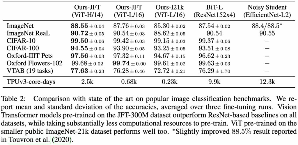
ViT models pre-trained on medium-scale datasets such as ImageNet-1k performed worse than ResNet models of comparable size. This is because CNNs are equipped with strong inductive biases such as translation equivariance and locality, which help them learn effectively from limited data. In contrast, ViT must learn such properties directly from data, which results in lower data efficiency.
However, when pre-trained on large-scale datasets such as ImageNet-21k or JFT-300M, ViT models outperform ResNets after being fine-tuned on target tasks.
Implementation
Patch Embedding
This module takes an input image and produces patch embeddings. First, the image is split into patches. Each patch is then flattened into a one-dimensional vector and projected into a -dimensional embedding space through a learnable linear projection. This process is functionally equivalent to what a convolutional layer performs.
Learnable linear projection can be implemented by a convolutional layer.
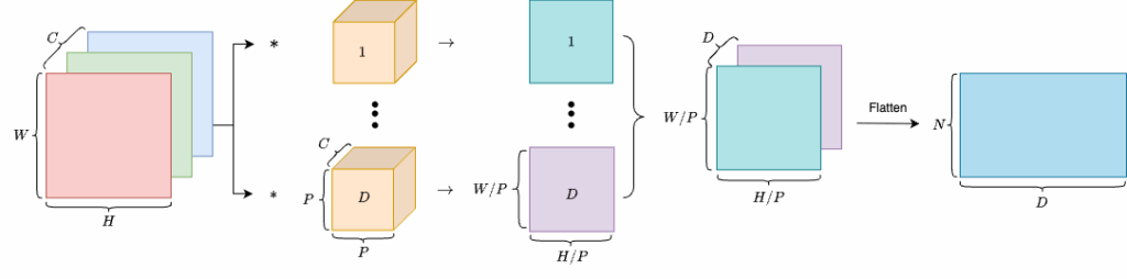
Thus, we can use a convolutional layer to transform an image of shape  into
into  , then flatten it to obtain a tensor of shape
  , where
  . Finally, we transpose the dimensions to get a tensor of shape
  .
.
class PatchEmbedding(nn.Module):
    def __init__(self, patch_size=16, in_channels=3, embed_dim=768):
        """
        Patch Embedding Layer for Vision Transformer.

        Args:
            patch_size (int): Size of the patches to be extracted from the input image.
            in_channels (int): Number of input channels in the image (e.g., 3 for RGB).
            embed_dim (int): Dimension of the embedding space to which each patch will be projected.
        """

        super(PatchEmbedding, self).__init__()
        self.patch_size = patch_size
        self.proj = nn.Conv2d(
            in_channels=in_channels,
            out_channels=embed_dim,
            kernel_size=patch_size,
            stride=patch_size,
        )

    def forward(self, x):
        """
        Forward pass of the Patch Embedding Layer.

        Args:
            x (torch.Tensor): Input tensor of shape (B, C, H, W) where
                                - B is batch size
                                - C is number of channels
                                - H is height
                                - W is width

        Returns:
            x (torch.Tensor): Output tensor of shape (B, D, H/P, W/P) where
                                - D is the embedding dimension
                                - H/P and W/P are the height and width of the patches.
        """

        x = self.proj(x)  # (B, D, H/P, W/P)
        x = x.flatten(2)  # (B, D, H/P * W/P)
        x = x.transpose(1, 2)  # (B, H/P * W/P, D)
        return x
Transformer Encoder
The following section shows the implementation of each component of the Transformer encoder.
class MultiHeadSelfAttention(nn.Module):
    def __init__(self, dim, num_heads=12, qkv_bias=True, dropout=0.1, attention_dropout=0.1):
        """
        Multi-Head Self-Attention Layer.

        Args:
            dim (int): Dimension of the input features.
            num_heads (int): Number of attention heads.
            qkv_bias (bool): Whether to add a bias term to the query, key, and value projections.
            dropout (float): Dropout rate applied to the output of the MLP and attention layers.
            attention_dropout (float): Dropout rate applied to the attention weights.
        """

        super().__init__()
        self.num_heads = num_heads
        self.head_dim = dim // num_heads
        self.scale = self.head_dim ** -0.5  # Scaled Dot-Product Attention 中的 √d_k

        self.qkv = nn.Linear(dim, dim * 3, bias=qkv_bias)
        self.attention_dropout = nn.Dropout(attention_dropout)
        self.projection = nn.Linear(dim, dim)
        self.projection_dropout = nn.Dropout(dropout)

    def forward(self, x):
        """
        Forward pass of the Multi-Head Self-Attention Layer.

        Args:
            x (torch.Tensor): Input tensor of shape (B, N, D) where
                                - B is batch size
                                - N is the number of patches (or tokens)
                                - D is the embedding dimension

        Returns:
            out (torch.Tensor): Output tensor of shape (B, N, D) after applying multi-head self-attention.
        """

        B, N, C = x.shape

        qkv = self.qkv(x)  # (B, N, 3C)
        qkv = qkv.reshape(B, N, 3, self.num_heads, self.head_dim)  # (B, N, 3, H, D)
        qkv = qkv.permute(2, 0, 3, 1, 4)  # (3, B, H, N, D)
        q, k, v = qkv[0], qkv[1], qkv[2]

        # Scaled Dot-Product Attention
        attn = (q @ k.transpose(-2, -1)) * self.scale  # (B, H, N, N)
        attn = attn.softmax(dim=-1)
        attn = self.attention_dropout(attn)

        out = (attn @ v)  # (B, H, N, D)
        out = out.transpose(1, 2).reshape(B, N, C)  # (B, N, D)
        out = self.projection(out)
        out = self.projection_dropout(out)
        return out
class MLPBlock(nn.Module):
def __init__(self, in_dim, hidden_dim, dropout=0.1):
"""
MLP Block for Transformer Encoder.
Args:
in_dim (int): Input dimension of the features.
hidden_dim (int): Hidden dimension of the MLP.
dropout (float): Dropout rate applied to the output of the MLP.
"""
super().__init__()
self.fc1 = nn.Linear(in_dim, hidden_dim)
self.act = nn.GELU()
self.fc2 = nn.Linear(hidden_dim, in_dim)
self.drop = nn.Dropout(dropout)
def forward(self, x):
"""
Forward pass of the MLP Block.
Args:
x (torch.Tensor): Input tensor of shape (B, N, D) where
- B is batch size
- N is the number of patches (or tokens)
- D is the embedding dimension
Returns:
x (torch.Tensor): Output tensor of the same shape as input, after applying MLP.
"""
x = self.fc1(x)
x = self.act(x)
x = self.drop(x)
x = self.fc2(x)
x = self.drop(x)
return xclass EncoderBlock(nn.Module):
def __init__(self, dim, num_heads, mlp_ratio=4.0, qkv_bias=True, dropout=0.1, attention_dropout=0.1):
"""
Transformer Encoder Block.
Args:
dim (int): Dimension of the input features.
num_heads (int): Number of attention heads.
mlp_ratio (float): Ratio of the hidden dimension in the MLP block to the embedding dimension.
qkv_bias (bool): Whether to add a bias term to the query, key, and value projections.
dropout (float): Dropout rate applied to the output of the MLP and attention layers.
attention_dropout (float): Dropout rate applied to the attention weights.
"""
super().__init__()
self.norm1 = nn.LayerNorm(dim)
self.self_attention = MultiHeadSelfAttention(
dim=dim,
num_heads=num_heads,
qkv_bias=qkv_bias,
dropout=dropout,
attention_dropout=attention_dropout,
)
self.norm2 = nn.LayerNorm(dim)
self.mlp = MLPBlock(
in_dim=dim,
hidden_dim=int(dim * mlp_ratio),
dropout=dropout,
)
def forward(self, x):
"""
Forward pass of the Transformer Encoder Block.
Args:
x (torch.Tensor): Input tensor of shape (B, N, D) where
- B is batch size
- N is the number of patches (or tokens)
- D is the embedding dimension
Returns:
x (torch.Tensor): Output tensor of the same shape as input, after applying self-attention and MLP.
"""
x = x + self.self_attention(self.norm1(x))
x = x + self.mlp(self.norm2(x))
return xVision Transformer
Below is the implementation of the Vision Transformer. It integrates the components described above. The image is first passed into the PatchEmbedding module to produce patch embeddings. A classification token is prepended to the sequence, followed by the addition of positional encodings. The cls_output, corresponding to , represents the final image representation.
In this implementation, we build a ViT for image classification. Therefore, a final linear projection maps the [CLS] token output to class logits. If the model is to be applied to a different task, this output head must be modified accordingly.
class VisionTransformer(nn.Module):
    def __init__(
        self,
        img_size=224,
        patch_size=16,
        in_channels=3,
        num_classes=1000,
        embed_dim=768,
        num_layers=12,
        num_heads=12,
        mlp_ratio=4.0,
        qkv_bias=True,
        dropout=0.1,
        attention_dropout=0.1,
    ):
        """
        Vision Transformer (ViT) model.

        Args:
            img_size (int): Size of the input image (assumed square).
            patch_size (int): Size of the patches to be extracted from the input image.
            in_channels (int): Number of input channels in the image (e.g., 3 for RGB).
            num_classes (int): Number of output classes for classification. If None, the model outputs the class token representation.
            embed_dim (int): Dimension of the embedding space to which each patch will be projected.
            num_layers (int): Number of Transformer encoder blocks.
            num_heads (int): Number of attention heads in the Multi-Head Self-Attention.
            mlp_ratio (float): Ratio of the hidden dimension in the MLP block to the embedding dimension.
            qkv_bias (bool): Whether to add a bias term to the query, key, and value projections.
            dropout (float): Dropout rate applied to the output of the MLP and attention layers.
            attention_dropout (float): Dropout rate applied to the attention weights.
        """

        super().__init__()

        self.patch_embedding = PatchEmbedding(patch_size, in_channels, embed_dim)
        num_patches = (img_size // patch_size) ** 2

        # Learnable Class Token
        self.cls_token = nn.Parameter(torch.zeros(1, 1, embed_dim))

        # Learnable Position Embedding: [cls_token, patch_1, ..., patch_N]
        self.positional_encoding = nn.Parameter(torch.zeros(1, num_patches + 1, embed_dim))
        self.pos_drop = nn.Dropout(p=dropout)

        self.blocks = nn.Sequential(*[
            EncoderBlock(
                dim=embed_dim,
                num_heads=num_heads,
                mlp_ratio=mlp_ratio,
                qkv_bias=qkv_bias,
                dropout=dropout,
                attention_dropout=attention_dropout,
            )
            for _ in range(num_layers)
        ])
        self.norm = nn.LayerNorm(embed_dim)

        self.head = nn.Identity() if num_classes is None else nn.Linear(embed_dim, num_classes)

        # Initialize parameters
        nn.init.trunc_normal_(self.positional_encoding, std=0.02)
        nn.init.trunc_normal_(self.cls_token, std=0.02)
        nn.init.trunc_normal_(self.head.weight, std=0.02)
        nn.init.zeros_(self.head.bias)

    def forward(self, x):
        """
        Forward pass of the Vision Transformer.

        Args:
            x (torch.Tensor): Input tensor of shape (B, C, H, W) where
                                - B is batch size
                                - C is number of channels
                                - H is height
                                - W is width

        Returns:
            logits (torch.Tensor): Output tensor of shape (B, num_classes) if num_classes is specified,
                                   otherwise the output is the class token representation of shape (B, D).
        """

        B = x.shape[0]

        x = self.patch_embedding(x)  # shape: (B, N, D)

        # Prepend a class token
        cls_tokens = self.cls_token.expand(B, -1, -1)  # (B, 1, D)
        x = torch.cat((cls_tokens, x), dim=1)  # (B, 1+N, D)

        x = x + self.positional_encoding  # (B, 1+N, D)
        x = self.pos_drop(x)  # (B, 1+N, D)

        x = self.blocks(x)  # (B, 1+N, D)
        x = self.norm(x)  # (B, 1+N, D)

        cls_output = x[:, 0]  # (B, D)

        logits = self.head(cls_output)  # (B, num_classes) or (B, D) if num_classes is None
        return logits
Pre-training and Inference
Using the VisionTransformer we just implemented, we build a cat-vs-dog image classifier. The following code shows the pre-training procedure.
class DogCatDataset(Dataset):
    def __init__(self, data_dir: Path, image_size=224):
        self.num_classes = 2  # 0 for dog, 1 for cat
        self.image_paths = list(data_dir.glob("*.png"))
        self.transform = T.Compose([
            T.ToTensor(),
            T.Resize((image_size, image_size))
        ])

    def __len__(self):
        return len(self.image_paths) * 2

    def __getitem__(self, idx):
        base_idx = idx // 2
        flip = idx % 2 == 1

        image_path = self.image_paths[base_idx]
        image = Image.open(image_path).convert("RGB")

        if flip:
            image = ImageOps.mirror(image)

        image = self.transform(image)
        label = 0 if "dog" in image_path.name.lower() else 1
        return image, label


device = torch.device("cuda" if torch.cuda.is_available() else "cpu")


def pretrain():
    model = VisionTransformer(embed_dim=768, num_classes=1000).to(device)

    dataset = DogCatDataset(data_dir=Path(__file__).parent.parent / "data" / "train")
    dataloader = DataLoader(dataset, batch_size=20, shuffle=True)

    EPOCHS = 50
    optimizer = torch.optim.AdamW(model.parameters(), lr=1e-3, weight_decay=0.01)
    criterion = torch.nn.CrossEntropyLoss()

    model.train()
    for epoch in range(EPOCHS):
        for images, labels in dataloader:
            images, labels = images.to(device), labels.to(device)
            logits = model(images)
            loss = criterion(logits, labels)

            optimizer.zero_grad()
            loss.backward()
            optimizer.step()

            print(f"Epoch {epoch} Loss: {loss.item():.4f}")

    return model
Once pre-training is complete, we can use the model to classify images, as shown below.
def inference(model):
    model.eval()
    transform = T.Compose([
        T.Resize((224, 224)),
        T.ToTensor(),
    ])

    cat_image = Image.open(Path(__file__).parent.parent / "data" / "val" / "cat-val.png").convert("RGB")
    cat_image_tensor = transform(cat_image).unsqueeze(0).to(device)

    dog_image = Image.open(Path(__file__).parent.parent / "data" / "val" / "dog-val.png").convert("RGB")
    dog_image_tensor = transform(dog_image).unsqueeze(0).to(device)

    with torch.no_grad():
        logits = model(cat_image_tensor)
        probs = F.softmax(logits, dim=-1)
        pred = probs.argmax(dim=-1).item()
        print(f"Predicted class index for cat: {pred} (should be 1)")

        logits = model(dog_image_tensor)
        probs = F.softmax(logits, dim=-1)
        pred = probs.argmax(dim=-1).item()
        print(f"Predicted class index for dog: {pred} (should be 0)")


if __name__ == "__main__":
    model = pretrain()
    inference(model)
    torch.save(model.state_dict(), "vit_dog_cat.pth")
    print("Model saved as vit_dog_cat.pth")
Conclusion
Vision Transformer introduces a new modeling paradigm in the visual domain. Its elegant and modular design challenges the long-standing dominance of CNN-based architectures. Although ViT has certain limitations in data- or compute-constrained settings, its success demonstrates the generality of the Transformer architecture and lays the foundation for subsequent developments in multimodal and self-supervised vision models such as DINO, BEiT, and CLIP. Future visual models may no longer rely on stacking convolutions, but instead build upon attention-based structural learning.
References
- Alexey Dosovitskiy, Lucas Beyer, Alexander Kolesnikov, Dirk Weissenborn, Xiaohua Zhai, Thomas Unterthiner, Mostafa Dehghani, Matthias Minderer, Georg Heigold, Sylvain Gelly, Jakob Uszkoreit, and Neil Houlsby. 2021. An Image Is Worth 16×16 Words: Transformers For Image Recognition at Scale. In 9th International Conference on Learning Representations, ICLR 2021.
- Source code, GitHub.


