時序差分學習（Temporal-Difference Learning, TD）

在強化學習中（Reinforcement Learning, RL），動態規劃（Dynamic Programming, DP）提供了最完整、最數學化的解法框架，但其對 environment model 的依賴，使其難以直接應用於真實環境；蒙地卡羅（Monte Carlo, MC）則能從經驗中學習，卻必須等待整個 episode 結束，更新粒度較為粗糙。時序差分（Temporal Difference, TD）正是介於兩者之間的一種折衷方法。它不需要已知的 model，卻能在每一步互動後即時更新估計值。

完整程式碼可以在下載。

增量式實作（Incremental Implementation）

在開始之前，我們必須要先了解增量式實作（incremental implementation）。若還不熟悉的話，可以先參考以下文章。

- Artificial Intelligence
- Reinforcement Learning

增量式實作（Incremental Implementation）

ByWayne
15/12/2025

時序差分（Temporal Difference, TD）

時序差分（Temporal Difference, TD）可視為動態規劃（Dynamic Programming, DP）和蒙地卡羅（Monte Carlo, MC）在概念上的結合。

如同 MC，TD 能夠直接從實際經驗中進行學習，而不需要事先知道 environment model。換言之，TD 屬於 model-free 方法。

同時，TD 也承襲了 DP 的特性，能夠利用目前的價值估計來更新價值估計本身，而不必等待整個 episode 結束或最終回報出現。TD 是 bootstrapping 方法。

時序差分預測（Temporal Difference Prediction）

單步時序差分（One-Step Temporal Difference, TD(0)）

在介紹 TD(0) 之前，我們先釐清 $v_\pi(s)$ 、 $v_*(s)$ 與 $V(s)$ 之間的差異。

$v_\pi(s)$ 表示在 policy $\pi$ 下，state $s$ 的 expected return。這是一個理論上的真值，而非估計值。在假設 environment model 已知的情況下，我們可以透過 Bellman expectation equation 精確計算 $v_\pi(s)$ ；若 model 未知，則 $v_\pi(s)$ 依然存在，但我們無法直接計算。

$v_(s)$ 則表示在最佳 policy 下，state $s$ 的 expected return。同樣地，這也是一個理論上的真值，而非估計值。即使我們不知道最佳 policy 為何， $v_(s)$ 仍然在數學上是定義良好的，只是無法直接計算。

$V(s)$ 則是 agent 在目前 policy 下，對 state $s$ 的 expected return 所形成的估計值。當 environment model 未知時，我們既無法計算 $v_\pi(s)$ ，也無法計算 $v_*(s)$ ，只能根據實際互動所蒐集到的資料，逐步學習並更新 $V(s)$ 。

以 every-visit MC 且使用常數步長（constant step size） $\alpha$ 為例，其 incremental update 形式為：

$V(S_t) \leftarrow V(S_t) + \alpha \big[ G_t - V(S_t) \big]$

MC 的特點在於，必須等待整個 episode 結束後，才能計算 return $G_t$ ，並據此更新 $V(S_t)$ 。

相較之下，TD 不需要等待 episode 結束。TD 在每一個 time step 後，即可利用當下觀察到的 reward $R_{t+1}$ ，以及下一個 state 的估計值 $V(S_{t+1})$ 來更新 $V(S_t)$ ：

$V(S_t) \leftarrow V(S_t) + \alpha \big[ R_{t+1} + \gamma V(S_{t+1}) - V(S_t) \big]$

這種方法稱為單步時序差分（one-step TD），亦即 TD(0)。

從 incremental update 的角度來看，DP 與 MC 所使用的 target 分別為：

$v_\pi(s) \doteq \mathbb{E}_\pi [ G_t \mid S_t=s ] \quad \text{... (MC)} \\\\ \hphantom{v_\pi(s)} = \mathbb{E}_\pi [ R_{t+1} + \gamma G_{t+1} \mid S_t=s ] \\\\ \hphantom{v_\pi(s)} = \mathbb{E}_\pi [ R_{t+1} + \gamma v_\pi(S_{t+1}) \mid S_t=s ] \quad \text{... (DP)}$

然而，TD 既無法計算 $v_\pi(S_{t+1})$ ，也不希望等待整個 episode 結束來取得 $G_t$ 。因此，TD 以實際觀察到的 reward $R_{t+1}$ ，搭配下一個 state 的估計值 $V(S_{t+1})$ ，來近似 return $G_t$ ：

$V(S_t) \leftarrow V(S_t) + \alpha [G_t - V(S_t)] ,\quad \text{ ...(MC)} \\\\ G_t \approx R_{t+1} + \gamma V(S_{t+1}) \\\\ V(S_t) \leftarrow V(S_t) + \alpha [R_{t+1} + \gamma V(S_{t+1}) - V(S_t)] ,\quad \text{ ...(TD)}$

其中括號中的數量是一種誤差，是測量 $S_t$ 的估計值與更新好的估計值 $R_{t+1} + \gamma V(S_{t+1})$ 之間的差異。這個誤差稱為 TD 誤差（TD error）。

其中，括號內的量衡量的是目前估計值 $V(S_t)$ ，與更新目標 $R_{t+1} + \gamma V(S_{t+1})$ 之間的差異。這個差異稱為時序差分誤差（TD error）：

$\delta_t \doteq R_{t+1} + \gamma V(S_{t+1}) - V(S_t)$

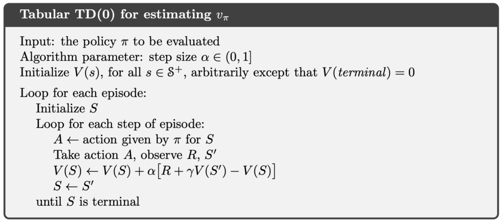
以下將介紹表格式（tabular）TD(0) prediction 的完整演算法。

Tabular TD(0) (source: Reinforcement Learning: An Introduction, 2nd).

時序差分控制（Temporal Difference Control）

Sarsa（On-Policy Temporal Difference Control）

我們可以將前一節介紹的 TD(0) prediction 延伸至 control 問題。如同 Monte Carlo（MC），TD 屬於 model-free 方法，並未假設已知 transition dynamics $p(s^\prime, r \mid s, a)$ 。因此，TD 無法像 DP 那樣，對 action 的結果進行期望值計算。

然而，透過與 environment 的實際互動，agent 所蒐集到的經驗中，包含了真實執行過的狀態與動作配對 $(s, a)$ ，以及對應的 reward 與下一個 state。這些樣本可用來直接估計 action 所帶來的回報。

因此，與 MC control 相同，TD control 不再直接對 state-value function $v_\pi(s)$ 進行操作，而是改為學習 action-value function $q_\pi(s, a)$ 。在此設定下，TD control 的更新規則為：

$Q(S_t, A_t) \leftarrow Q(S_t, A_t) + \alpha [R_{t+1} + \gamma Q(S_{t+1}, A_{t+1}) - Q(S_t, A_t)]$

此更新會在每一次狀態轉移後立即進行，而不需要等待 episode 結束。更新式中所使用的五個元素 $S_t, A_t, R_{t+1}, S_{t+1}, A_{t+1}$ ，正好對應到一次完整的互動樣本，因此該演算法被稱為 Sarsa。

由於下一個 action $A_{t+1}$ 是依照目前正在執行的 policy 所選擇，Sarsa 屬於一種 on-policy TD control。

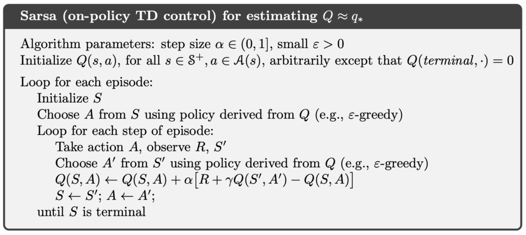
以下為 Sarsa 演算法的完整流程。

Sarsa, On-Policy TD Control (source: Reinforcement Learning: An Introduction, 2nd).

Q-Learning（Off-Policy Temporal Difference Control）

相較於 Sarsa，Q-Learning 在更新時，並不使用實際執行的下一個 action，而是直接以下一個 state 下的最佳 action 作為更新目標。換言之，Q-Learning 的更新目標近似於 optimal action-value function $q_*$ 。其更新式如下：

$\displaystyle Q(S_t, A_t) \leftarrow Q(S_t, A_t) + \alpha [R_{t+1} + \gamma \max_a Q(S_{t+1}, a) - Q(S_t, A_t)]$

與 Sarsa 不同，Q-Learning 在更新時，並不關心 agent 在下一個 state $S_{t+1}$ 實際採取了哪一個 action，而是直接假設 agent 將選擇當下估計值最大的 action。這使得 Q-Learning 在學習過程中，行為策略（behavior policy）與更新的目標策略（target policy）可以不同。

因此，Q-Learning 屬於一種 off-policy 的 TD control。在實務上，agent 可以使用具有探索性的 behavior policy（例如， $\varepsilon$ -greedy）與 environment 互動，但在更新時，始終朝向 greedy policy 所對應的 $q_*$ 進行學習。

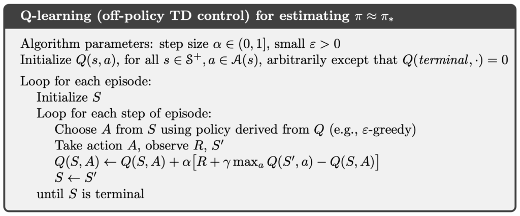
以下為 Q-Learning 演算法的完整流程。

Q-Learning, Off-Policy TD Control (source: Reinforcement Learning: An Introduction, 2nd).

Expected Sarsa（On-Policy/Off-Policy Temporal Difference Control）

相較於 Sarsa 使用實際執行的下一個 action $Q(S_{t+1}, A_{t+1})$ ，以及 Q-Learning 使用下一個 state 下的最大 action-value $\max_a Q(S_{t+1}, a)$ ，Expected Sarsa 則直接對下一個 state 的 action-value 取期望值，其更新式如下：

$\displaystyle Q(S_t, A_t) \leftarrow Q(S_t, A_t) + \alpha [R_{t+1} + \gamma \mathbb{E}_\pi [Q(S_{t+1}, A_{t+1}) \mid S_{t+1}] - Q(S_t, A_t)] \\\\ \hphantom{Q(S_t, A_t)} \leftarrow Q(S_t, A_t) + \alpha [R_{t+1} + \gamma \sum_a \pi(a \mid S_{t+1}) Q(S_{t+1}, a) - Q(S_t, A_t)]$

透過明確地引入 policy $\pi$ 對 action 的期望值，Expected Sarsa 在更新目標的定義上，介於 Sarsa 與 Q-learning 之間。當 policy $\pi$ 採用 $\varepsilon$ -greedy 形式，且 $\varepsilon$ 較大時，期望值中會顯著反映探索行為的影響，此時 Expected Sarsa 屬於 on-policy 方法，並展現出與 Sarsa 類似、偏向保守的行為。

隨著 $\varepsilon$ 逐漸減小， $\varepsilon$ -greedy policy 會趨近於 greedy policy，探索風險在期望值中的影響也隨之降低。若在此同時，behavior policy 仍保有探索性，則用於取期望的 policy 與實際行為的 policy 便產生不一致，使 Expected Sarsa 轉為 off-policy 方法。在這種設定下，其更新目標將逐漸接近 Q-learning 的形式，因此可視為對 Q-learning 的一種連續化與泛化。

除了些微增加的計算成本之外，Expected Sarsa 通常能在學習穩定性與收斂效率之間取得良好的平衡，因此在實務上，常被視為一種同時涵蓋並改進 Sarsa 與 Q-Learning 的 TD control 方法。

Sarsa 範例

Sarsa 實作

在以下的程式碼，我們忠實地實作 Sarsa 方法。

程式碼中的 env 是 Gymnasium 的 Env 物件。Gymnasium 的前身是 OpenAI Gym。它提供了眾多的 RL 環境的數據，讓我們可以在模擬的環境中，測試 RL 演算法。

Environment 中有 env.observation_space.n 個 states。因此，state 的編號就從整數 0 到 env.observation_space.n - 1。變數 Q 是一個浮點數的 2D-array，每一個 element 都是一對 state 和 action 的 action-value 的估計值。例如，Q[0][0] 是 state 0 的 action 0 的 action-value 估計值。

import gymnasium as gym
import numpy as np


class Sarsa:
    def __init__(self, env: gym.Env, alpha=0.5, gamma=1.0, epsilon=0.1):
        self.env = env
        self.alpha = alpha
        self.gamma = gamma
        self.epsilon = epsilon

    def _random_argmax(self, q_s: np.ndarray) -> int:
        ties = np.flatnonzero(np.isclose(q_s, q_s.max()))
        return np.random.choice(ties)

    def _epsilon_greedy_action(self, Q: np.ndarray, s: int) -> int:
        if np.random.rand() < self.epsilon:
            return np.random.choice(self.env.action_space.n)
        else:
            ties = np.flatnonzero(np.isclose(Q[s], Q[s].max()))
            return np.random.choice(ties)

    def _create_pi_by_Q(self, Q: np.ndarray) -> np.ndarray:
        pi = np.zeros((self.env.observation_space.n, self.env.action_space.n), dtype=float)
        for s in range(self.env.observation_space.n):
            A_start = self._random_argmax(Q[s])
            pi[s][A_start] = 1.0
        return pi

    def run_control(self, n_episodes=5000) -> tuple[np.ndarray, np.ndarray]:
        Q = np.zeros((self.env.observation_space.n, self.env.action_space.n), dtype=float)

        for i_episode in range(1, n_episodes + 1):
            print(f"\rEpisode: {i_episode}/{n_episodes}", end="", flush=True)

            s, _ = self.env.reset()
            a = self._epsilon_greedy_action(Q, s)

            terminated = False
            truncated = False
            while not (terminated or truncated):
                s_prime, r, terminated, truncated, _ = self.env.step(a)
                a_prime = self._epsilon_greedy_action(Q, s_prime)
                if terminated or truncated:
                    Q[s, a] = Q[s, a] + self.alpha * (r + self.gamma * 0 - Q[s, a])
                else:
                    Q[s, a] = Q[s, a] + self.alpha * (r + self.gamma * Q[s_prime, a_prime] - Q[s, a])
                s = s_prime
                a = a_prime

        pi = self._create_pi_by_Q(Q)
        print()
        return pi, Q

Cliff Walking

Cliff Walking 涉及在一個網格世界（grid world）中，從起始位置移動到目標位置，同時避免掉落懸崖，如下圖。

Cliff Walking 問題中每個 state 就是玩家的目前的 position。因此共有 36 個 states，分別是上面三排加上左下的格子， $3 * 12 + 1 = 36$ 。目前的 position 由以下公式算出：

$\text{position} = \text{current-row} \times \text{num-col} + \text{current-col}$

有四個 actions，分別是：

0：Move up
1：Move right
2：Move down
3：Move left

每一步皆給予 −1 reward。但若玩家踏入懸崖（cliff），則會受到 −100 reward。

import time

import gymnasium as gym
import numpy as np

from expected_sarsa import ExpectedSarsa
from q_learning import QLearning
from sarsa import Sarsa

GYM_ID = "CliffWalking-v1"


def play_game(policy, episodes=1):
    visual_env = gym.make(GYM_ID, render_mode="human")

    for episode in range(episodes):
        state, _ = visual_env.reset()
        terminated = False
        truncated = False
        total_reward = 0
        step_count = 0

        for i in range(10):
            print(f"Sleep {i}")
            time.sleep(1)

        print(f"Episode {episode + 1} starts")
        while not terminated and not truncated:
            action = np.argmax(policy[state])
            state, reward, terminated, truncated, _ = visual_env.step(action)
            total_reward += reward
            step_count += 1
            time.sleep(0.3)

        print(f"Episode {episode + 1} is finished: Total reward is {total_reward}, steps = {step_count}")
        time.sleep(1)

    visual_env.close()


if __name__ == "__main__":
    env = gym.make(GYM_ID)

    print(f"Gym environment: {GYM_ID}")

    print("Start Sarsa")
    sarsa = Sarsa(env)
    sarsa_policy, sarsa_Q = sarsa.run_control()
    play_game(sarsa_policy)
    print("\n")

    env.close()

以下是以上程式的執行結果。可以觀察到，agent 並未選擇貼近懸崖的最短路徑，而是傾向於採取距離懸崖較遠、風險較低的路徑。這是因為 Sarsa 在更新 action-value 時，使用的是由同一個 $\varepsilon$ -greedy policy 所實際採樣到的下一個 action，使得探索行為所帶來的風險會直接反映在價值估計中。因此，在 Cliff Walking 這類高風險環境下，Sarsa 自然會學到較為保守、但穩定的策略。

Taxi

Taxi 問題是在一個 grid world 中移動，前往乘客所在的位置接送乘客，並將乘客送達四個指定地點之一，如下圖。

Taxi 問題中有 500 個 discrete states。每個 state 由以下公式算出：

$r: \text{the row the taxi is currently at} \\\\ c: \text{the colunm the taxi is currently at} \\\\ p: \text{the location the passenger is at} \\\\ d: \text{the destination to drop off the passenger} \\\\ state = ((r \times 5 + c) \times 5 + p) * 4 + d$

Passenger 的 locations：

0：Red
1：Green
2：Yellow
3：Blue
4：In taxi

Destinations：

0：Red
1：Green
2：Yellow
3：Blue

有六個 actions，分別是：

0：Move south（down）
1：Move north（up）
2：Move east（right）
3：Move west（left）
4：Pickup passenger
5：Drop off passenger

每一步皆給予 −1 reward，除非觸發其他 reward。成功將乘客送達目的地可獲得 +20 reward。非法執行 pickup 或 drop-off 動作時，會受到 −10 reward。

import time

import gymnasium as gym
import numpy as np

from expected_sarsa import ExpectedSarsa
from q_learning import QLearning
from sarsa import Sarsa

GYM_ID = "Taxi-v3"


def play_game(policy, episodes=1):
    visual_env = gym.make(GYM_ID, render_mode="human")

    for episode in range(episodes):
        state, _ = visual_env.reset()
        terminated = False
        truncated = False
        total_reward = 0
        step_count = 0

        for i in range(10):
            print(f"Sleep {i}")
            time.sleep(1)

        print(f"Episode {episode + 1} starts")
        while not terminated and not truncated:
            action = np.argmax(policy[state])
            state, reward, terminated, truncated, _ = visual_env.step(action)
            total_reward += reward
            step_count += 1
            time.sleep(0.3)

        print(f"Episode {episode + 1} is finished: Total reward is {total_reward}, steps = {step_count}")
        time.sleep(1)

    visual_env.close()


if __name__ == "__main__":
    env = gym.make(GYM_ID)

    print(f"Gym environment: {GYM_ID}")

    print("Start Sarsa")
    sarsa = Sarsa(env)
    sarsa_policy, sarsa_Q = sarsa.run_control()
    play_game(sarsa_policy)
    print("\n")

    env.close()

以下是上面程式的執行結果。

Q-Learning 範例

Q-Learning 實作

在以下的程式碼，我們忠實地實作 Q-Learning 方法。

import gymnasium as gym
import numpy as np


class QLearning:
    def __init__(self, env: gym.Env, alpha=0.5, gamma=1.0, epsilon=0.1):
        self.env = env
        self.alpha = alpha
        self.gamma = gamma
        self.epsilon = epsilon

    def _random_argmax(self, q_s: np.ndarray) -> int:
        ties = np.flatnonzero(np.isclose(q_s, q_s.max()))
        return np.random.choice(ties)

    def _epsilon_greedy_action(self, Q: np.ndarray, s: int) -> int:
        if np.random.rand() < self.epsilon:
            return np.random.choice(self.env.action_space.n)
        else:
            ties = np.flatnonzero(np.isclose(Q[s], Q[s].max()))
            return np.random.choice(ties)

    def _create_pi_by_Q(self, Q: np.ndarray) -> np.ndarray:
        pi = np.zeros((self.env.observation_space.n, self.env.action_space.n), dtype=float)
        for s in range(self.env.observation_space.n):
            A_start = self._random_argmax(Q[s])
            pi[s][A_start] = 1.0
        return pi

    def run_control(self, n_episode=5000) -> tuple[np.ndarray, np.ndarray]:
        Q = np.zeros((self.env.observation_space.n, self.env.action_space.n), dtype=float)

        for i_episode in range(1, n_episode + 1):
            print(f"\rEpisode: {i_episode}/{n_episode}", end="", flush=True)

            s, _ = self.env.reset()

            terminated = False
            truncated = False
            while not (terminated or truncated):
                a = self._epsilon_greedy_action(Q, s)
                s_prime, r, terminated, truncated, _ = self.env.step(a)
                if terminated or truncated:
                    Q[s, a] = Q[s, a] + self.alpha * (r + self.gamma * 0 - Q[s, a])
                else:
                    Q[s, a] = Q[s, a] + self.alpha * (r + self.gamma * np.max(Q[s_prime]) - Q[s, a])
                s = s_prime

        pi = self._create_pi_by_Q(Q)
        print()
        return pi, Q

Cliff Walking

以下我們用 Q-Learning 來解決 Cliff Walking 問題。

import time

import gymnasium as gym
import numpy as np

from expected_sarsa import ExpectedSarsa
from q_learning import QLearning
from sarsa import Sarsa

GYM_ID = "CliffWalking-v1"


def play_game(policy, episodes=1):
    visual_env = gym.make(GYM_ID, render_mode="human")

    for episode in range(episodes):
        state, _ = visual_env.reset()
        terminated = False
        truncated = False
        total_reward = 0
        step_count = 0

        for i in range(10):
            print(f"Sleep {i}")
            time.sleep(1)

        print(f"Episode {episode + 1} starts")
        while not terminated and not truncated:
            action = np.argmax(policy[state])
            state, reward, terminated, truncated, _ = visual_env.step(action)
            total_reward += reward
            step_count += 1
            time.sleep(0.3)

        print(f"Episode {episode + 1} is finished: Total reward is {total_reward}, steps = {step_count}")
        time.sleep(1)

    visual_env.close()


if __name__ == "__main__":
    env = gym.make(GYM_ID)

    print(f"Gym environment: {GYM_ID}")

    print("Start Q-learning")
    q_learning = QLearning(env)
    ql_policy, ql_Q = q_learning.run_control()
    play_game(ql_policy)
    print("\n")

    env.close()

以下是以上程式的執行結果。可以觀察到，agent 會學到貼近懸崖的最短路徑，因為 Q-learning 在更新 action-value 時，使用的是 $\max_a Q(S_{t+1}, a)$ 作為 TD target，而不考慮實際探索行為所帶來的風險。這使得 Q-learning 直接逼近 optimal action-value function $q_*$ ，在評估階段表現出較高的效率，但在訓練過程中則更容易因探索而掉入懸崖。

Taxi

以下我們用 Q-Learning 來解決 Taxi 問題。

import time

import gymnasium as gym
import numpy as np

from expected_sarsa import ExpectedSarsa
from q_learning import QLearning
from sarsa import Sarsa

GYM_ID = "Taxi-v3"


def play_game(policy, episodes=1):
    visual_env = gym.make(GYM_ID, render_mode="human")

    for episode in range(episodes):
        state, _ = visual_env.reset()
        terminated = False
        truncated = False
        total_reward = 0
        step_count = 0

        for i in range(10):
            print(f"Sleep {i}")
            time.sleep(1)

        print(f"Episode {episode + 1} starts")
        while not terminated and not truncated:
            action = np.argmax(policy[state])
            state, reward, terminated, truncated, _ = visual_env.step(action)
            total_reward += reward
            step_count += 1
            time.sleep(0.3)

        print(f"Episode {episode + 1} is finished: Total reward is {total_reward}, steps = {step_count}")
        time.sleep(1)

    visual_env.close()


if __name__ == "__main__":
    env = gym.make(GYM_ID)

    print(f"Gym environment: {GYM_ID}")

    print("Start Q-learning")
    q_learning = QLearning(env)
    ql_policy, ql_Q = q_learning.run_control()
    play_game(ql_policy)
    print("\n")

    env.close()

以下是上面程式的執行結果。

Expected Sarsa 範例

Expected Sarsa 實作

在以下的程式碼，我們忠實地實作 Expected Sarsa 方法。

import gymnasium as gym
import numpy as np


class ExpectedSarsa:
    def __init__(self, env: gym.Env, alpha=0.5, gamma=1.0, epsilon=0.1):
        self.env = env
        self.alpha = alpha
        self.gamma = gamma
        self.epsilon = epsilon

    def _random_argmax(self, q_s: np.ndarray) -> int:
        ties = np.flatnonzero(np.isclose(q_s, q_s.max()))
        return np.random.choice(ties)

    def _epsilon_greedy_action(self, Q: np.ndarray, s: int) -> int:
        if np.random.rand() < self.epsilon:
            return np.random.choice(self.env.action_space.n)
        else:
            ties = np.flatnonzero(np.isclose(Q[s], Q[s].max()))
            return np.random.choice(ties)

    def _epsilon_greedy_probabilities(self, q_s: np.ndarray):
        probs = np.ones(self.env.action_space.n, dtype=float) * (self.epsilon / self.env.action_space.n)
        max_q = np.max(q_s)
        greedy_actions = np.flatnonzero(np.isclose(q_s, max_q))
        probs[greedy_actions] += (1 - self.epsilon) / len(greedy_actions)
        return probs

    def _create_pi_by_Q(self, Q: np.ndarray) -> np.ndarray:
        pi = np.zeros((self.env.observation_space.n, self.env.action_space.n), dtype=float)
        for s in range(self.env.observation_space.n):
            A_start = self._random_argmax(Q[s])
            pi[s][A_start] = 1.0
        return pi

    def run_control(self, n_episodes=5000):
        Q = np.zeros((self.env.observation_space.n, self.env.action_space.n), dtype=float)

        for i_episode in range(1, n_episodes + 1):
            print(f"\rEpisode: {i_episode}/{n_episodes}", end="", flush=True)

            s, _ = self.env.reset()

            terminated = False
            truncated = False
            while not (terminated or truncated):
                a = self._epsilon_greedy_action(Q, s)
                s_prime, r, terminated, truncated, _ = self.env.step(a)
                if terminated or truncated:
                    Q[s, a] = Q[s, a] + self.alpha * (r + self.gamma * 0 - Q[s, a])
                else:
                    expectation = np.dot(self._epsilon_greedy_probabilities(Q[s_prime]), Q[s_prime])
                    Q[s, a] = Q[s, a] + self.alpha * (r + self.gamma * expectation - Q[s, a])
                s = s_prime

        pi = self._create_pi_by_Q(Q)
        print()
        return pi, Q

Cliff Walking

以下我們用 Expected Sarsa 來解決 Cliff Walking 問題。我們分別執行了 $latax \varepsilon=0.1$ 和 $\varepsilon=0.001$ 。

import time

import gymnasium as gym
import numpy as np

from expected_sarsa import ExpectedSarsa
from q_learning import QLearning
from sarsa import Sarsa

GYM_ID = "CliffWalking-v1"


def play_game(policy, episodes=1):
    visual_env = gym.make(GYM_ID, render_mode="human")

    for episode in range(episodes):
        state, _ = visual_env.reset()
        terminated = False
        truncated = False
        total_reward = 0
        step_count = 0

        for i in range(10):
            print(f"Sleep {i}")
            time.sleep(1)

        print(f"Episode {episode + 1} starts")
        while not terminated and not truncated:
            action = np.argmax(policy[state])
            state, reward, terminated, truncated, _ = visual_env.step(action)
            total_reward += reward
            step_count += 1
            time.sleep(0.3)

        print(f"Episode {episode + 1} is finished: Total reward is {total_reward}, steps = {step_count}")
        time.sleep(1)

    visual_env.close()


if __name__ == "__main__":
    env = gym.make(GYM_ID)

    print(f"Gym environment: {GYM_ID}")

    print("Start Expected Sarsa with epsilon = 0.1")
    esarsa_01 = ExpectedSarsa(env, epsilon=0.1)
    esarsa_01_policy, esarsa_01_Q = esarsa_01.run_control()
    play_game(esarsa_01_policy)
    print("\n")

    print("Start Expected Sarsa with epsilon = 0.001")
    esarsa_0001 = ExpectedSarsa(env, epsilon=0.001)
    esarsa_0001_policy, esarsa_0001_Q = esarsa_0001.run_control()
    play_game(esarsa_0001_policy)
    print("\n")

    env.close()

以下是以上程式的執行結果。與 Sarsa 與 Q-learning 不同，Expected Sarsa 在更新 action-value 時，會對下一個 state 下所有可能 action 的價值取期望，因此能夠將探索行為的風險平均地納入考量。

當 $\varepsilon$ 較大時（如：0.1），這代表 agent 意識到自己走路常常滑倒（10% 機率）於是傾向於選擇離懸崖遠一點的安全路徑。而當 $\varepsilon$ 非常小時（如：0.001），這代表 agent 想自己走路幾乎不會滑倒（0.01% 機率），探索風險幾乎可以忽略，平均來看走懸崖邊緣還是最划算的，學到的行為也會開始貼近懸崖。

從這個角度來看，Expected Sarsa 的行為會隨著 $\varepsilon$ 的設定，在風險意識與效率優先之間平滑地轉換，正好形成 Sarsa 與 Q-learning 之間的自然折衷。

Cliff Walking by Expected Sarsa with epsilon 0.1.

Cliff Walking by Expected Sarsa with epsilon 0.001.

Taxi

以下我們用 Expected Sarsa 來解決 Cliff Walking 問題。我們分別執行了 $latax \varepsilon=0.1$ 和 $\varepsilon=0.001$ 。

import time

import gymnasium as gym
import numpy as np

from expected_sarsa import ExpectedSarsa
from q_learning import QLearning
from sarsa import Sarsa

GYM_ID = "Taxi-v3"


def play_game(policy, episodes=1):
    visual_env = gym.make(GYM_ID, render_mode="human")

    for episode in range(episodes):
        state, _ = visual_env.reset()
        terminated = False
        truncated = False
        total_reward = 0
        step_count = 0

        for i in range(10):
            print(f"Sleep {i}")
            time.sleep(1)

        print(f"Episode {episode + 1} starts")
        while not terminated and not truncated:
            action = np.argmax(policy[state])
            state, reward, terminated, truncated, _ = visual_env.step(action)
            total_reward += reward
            step_count += 1
            time.sleep(0.3)

        print(f"Episode {episode + 1} is finished: Total reward is {total_reward}, steps = {step_count}")
        time.sleep(1)

    visual_env.close()


if __name__ == "__main__":
    env = gym.make(GYM_ID)

    print(f"Gym environment: {GYM_ID}")

    print("Start Expected Sarsa with epsilon = 0.1")
    esarsa_01 = ExpectedSarsa(env, epsilon=0.1)
    esarsa_01_policy, esarsa_01_Q = esarsa_01.run_control()
    play_game(esarsa_01_policy)
    print("\n")

    print("Start Expected Sarsa with epsilon = 0.001")
    esarsa_0001 = ExpectedSarsa(env, epsilon=0.001)
    esarsa_0001_policy, esarsa_0001_Q = esarsa_0001.run_control()
    play_game(esarsa_0001_policy)
    print("\n")

    env.close()

以下是上面程式的執行結果。

Taxi by Expected Sarsa with epsilon 0.1.

Taxi by Expected Sarsa with epsilon 0.001.

結論

本章介紹了的 TD prediction 與三種 TD control 方法。我們可以發現它們在形式上雖然各異，但本質上皆建立在同一套 incremental update 框架之上。Sarsa、Q-learning 與 Expected Sarsa 的差異，並不在於學習流程本身，而在於對更新目標的定義方式，以及 on-policy 與 off-policy 的取捨。透過這樣的統一視角，TD control 不再是零散的演算法集合，而是一個連續且可互相對照的學習家族。

參考

Adam White and Martha White. Reinforcement Learning Specialization. University of Alberta and Coursera.
Richard S. Sutton and Andrew G. Barto. 2020. Reinforcement Learning: An Introduction, 2^nd. The MIT Press.

時序差分學習（Temporal-Difference Learning, TD）

Share

Table of Contents

增量式實作（Incremental Implementation）

時序差分（Temporal Difference, TD）

時序差分預測（Temporal Difference Prediction）

單步時序差分（One-Step Temporal Difference, TD(0)）

時序差分控制（Temporal Difference Control）

Sarsa（On-Policy Temporal Difference Control）

Q-Learning（Off-Policy Temporal Difference Control）

Expected Sarsa（On-Policy/Off-Policy Temporal Difference Control）

Sarsa 範例

Sarsa 實作

Cliff Walking

Taxi

Q-Learning 範例

Q-Learning 實作

Cliff Walking

Taxi

Expected Sarsa 範例

Expected Sarsa 實作

Cliff Walking

Taxi

結論

參考

Related Tags

發佈留言 取消回覆

You May Also Like

發佈留言取消回覆